05: Data Modeling

linear model

predictions

diagnostics

Author

Thomas Manke

Recap: All-Against-All Correlations

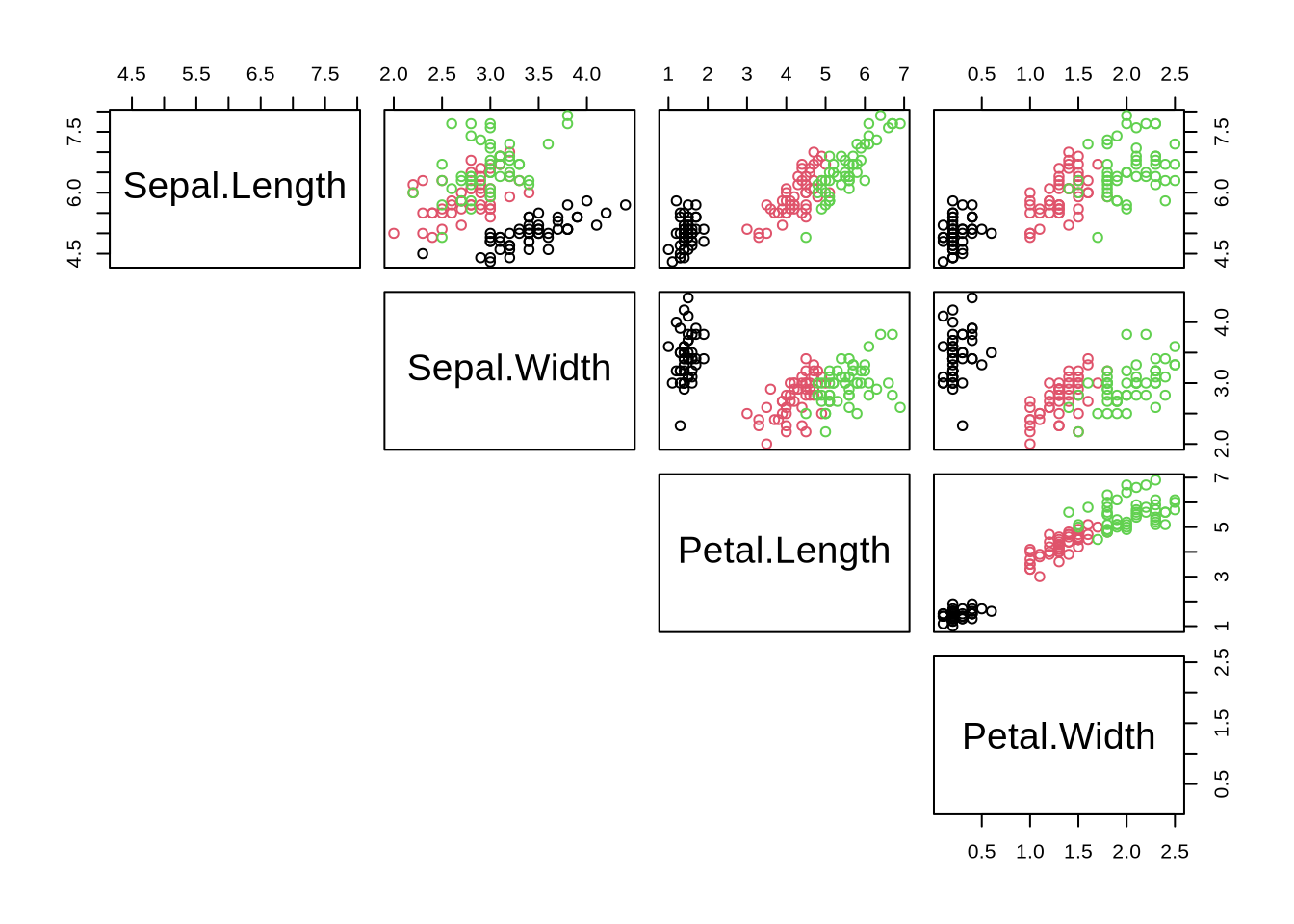
Task: Generate all-against-all correlation plot. Understand:

cols
selection/unselection of elements [,-5]
plot() function and arguments

Code

# assign species-colors to each observation 
cols = iris$Species                            # understand how color is defined
plot(iris[,-5], col=cols, lower.panel=NULL)   # "cols" was defined in task above

From Correlations to Models

Goal:

Model some dependent variable y as function of other explanatory variables x (features)

\[ y = f(\theta, x) = \theta_1 x + \theta_0 \]

For \(N\) data points, choose parameters \(\theta\) by ordinary least squares:

\[ RSS=\sum_{i=1}^{N} (y_i - f(\theta, x_i))^2 \to min \]

Easy in R:

Code

plot(Petal.Width ~ Petal.Length, data=iris, col=Species) # use model ("formula") notation
fit=lm(Petal.Width ~ Petal.Length, data=iris)       # fit a linear model
abline(fit, lwd=3, lty=2)                           # add regression line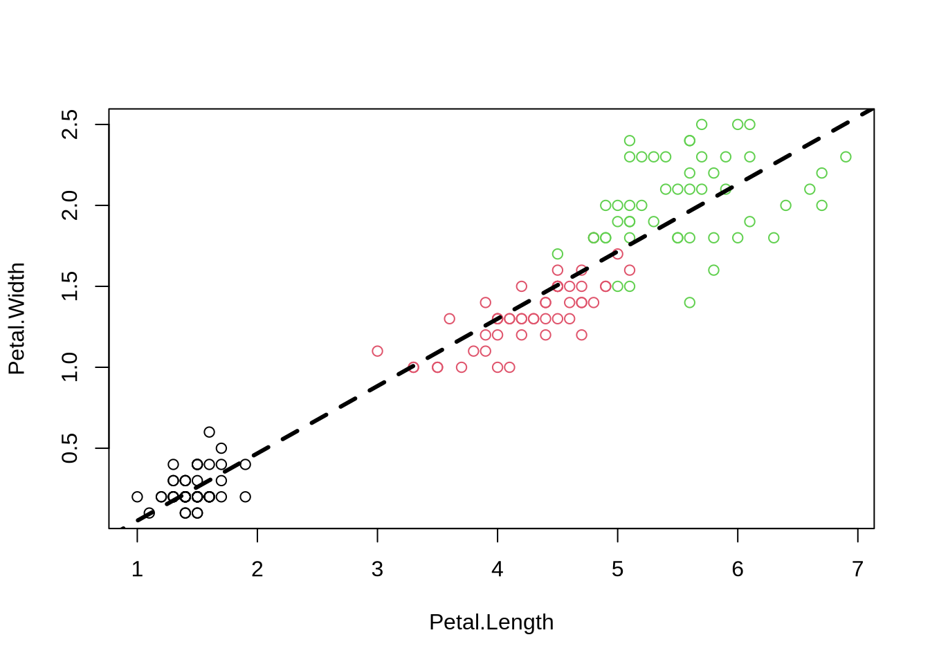

Query: What class is the object fit?

Task: Extract the coefficients of the fitted line.

 (Intercept) Petal.Length 
  -0.3630755    0.4157554

 (Intercept) Petal.Length 
  -0.3630755    0.4157554

There are many more methods to access information for the lm class

Code

methods(class='lm')

 [1] add1           alias          anova          case.names     coerce        
 [6] confint        cooks.distance deviance       dfbeta         dfbetas       
[11] drop1          dummy.coef     effects        extractAIC     family        
[16] formula        hatvalues      influence      initialize     kappa         
[21] labels         logLik         model.frame    model.matrix   nobs          
[26] plot           predict        print          proj           qr            
[31] residuals      rstandard      rstudent       show           simulate      
[36] slotsFromS3    summary        variable.names vcov          
see '?methods' for accessing help and source code

Reporting the fit (model)

Code

summary(fit)        # summary() behaves differently for fit objects


Call:
lm(formula = Petal.Width ~ Petal.Length, data = iris)

Residuals:
     Min       1Q   Median       3Q      Max 
-0.56515 -0.12358 -0.01898  0.13288  0.64272 

Coefficients:
              Estimate Std. Error t value Pr(>|t|)    
(Intercept)  -0.363076   0.039762  -9.131  4.7e-16 ***
Petal.Length  0.415755   0.009582  43.387  < 2e-16 ***
---
Signif. codes:  0 '***' 0.001 '**' 0.01 '*' 0.05 '.' 0.1 ' ' 1

Residual standard error: 0.2065 on 148 degrees of freedom
Multiple R-squared:  0.9271,    Adjusted R-squared:  0.9266 
F-statistic:  1882 on 1 and 148 DF,  p-value: < 2.2e-16

Code

coefficients(fit)   # more functions for specific elements

 (Intercept) Petal.Length 
  -0.3630755    0.4157554

Code

confint(fit)        # Try to change the confidence level: ?confint

                  2.5 %     97.5 %
(Intercept)  -0.4416501 -0.2845010
Petal.Length  0.3968193  0.4346915

This is a good fit as suggested by a

small residual standard error
a large coefficient of variation \(R^2\)
large F-statistics \(\to\) small p-value
and by visualization

Fraction of variation explained by model: \[ R^2 = 1 - \frac{RSS}{TSS} = 1 - \frac{\sum_i(y_i - y(\theta,x_i))^2}{\sum_i(y_i-\bar{y})^2} \]

Predictions (with confidence intervals)

Uncertainties in parameters become uncertainties in fits:

Code

x=iris$Petal.Length                       # explanatory variable from fit (here:Petal.Length)
xn=seq(min(x), max(x), length.out = 100)  # define range of new explanatory variables
ndf=data.frame(Petal.Length=xn)           # put them into new data frame

p=predict(fit, ndf, interval = 'confidence' , level = 0.95)
plot(Petal.Width ~ Petal.Length, data=iris, col=Species)
lines(xn, p[,"lwr"] )
lines(xn, p[,"upr"] )

#some fancy filling
polygon(c(rev(xn), xn), c(rev(p[ ,"upr"]), p[ ,"lwr"]), col = rgb(1,0,0,0.5), border = NA)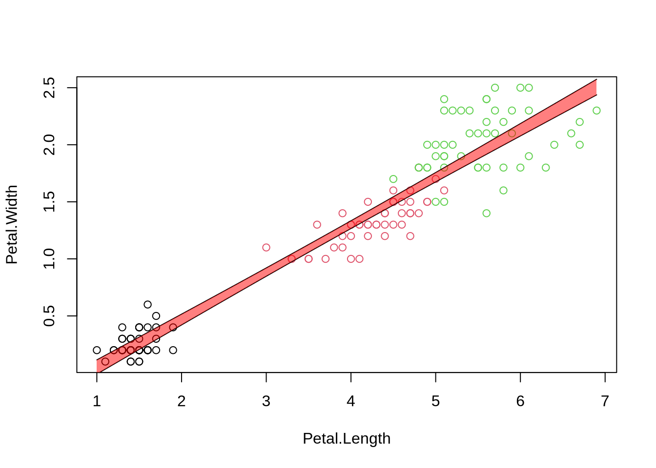

Code

## using ggplot2 - full introduction later
#library(ggplot2)
#g = ggplot(iris, aes(Petal.Length, Petal.Width, colour=Species))
#g + geom_point() + geom_smooth(method="lm", se=TRUE, color="red") + geom_smooth(method="loess", colour="blue")

Poor Model

Just replace “Petal” with “Sepal”

Code

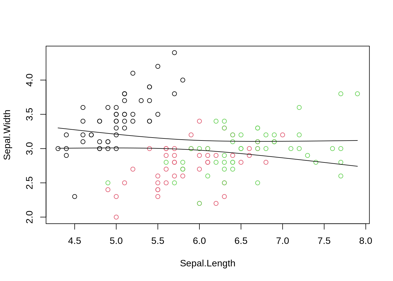
plot(Sepal.Width ~ Sepal.Length, data=iris, col=cols)  
fit1=lm(Sepal.Width ~ Sepal.Length, data=iris)     
abline(fit1, lwd=3, lty=2)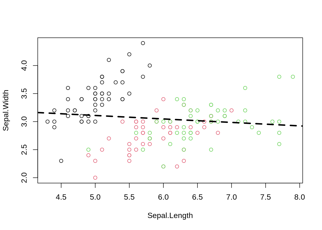

Code

confint(fit1)                     # estimated slope is indistinguishable from zero

                  2.5 %     97.5 %
(Intercept)   2.9178767 3.92001694
Sepal.Length -0.1467928 0.02302323

Code

summary(fit1)


Call:
lm(formula = Sepal.Width ~ Sepal.Length, data = iris)

Residuals:
    Min      1Q  Median      3Q     Max 
-1.1095 -0.2454 -0.0167  0.2763  1.3338 

Coefficients:
             Estimate Std. Error t value Pr(>|t|)    
(Intercept)   3.41895    0.25356   13.48   <2e-16 ***
Sepal.Length -0.06188    0.04297   -1.44    0.152    
---
Signif. codes:  0 '***' 0.001 '**' 0.01 '*' 0.05 '.' 0.1 ' ' 1

Residual standard error: 0.4343 on 148 degrees of freedom
Multiple R-squared:  0.01382,   Adjusted R-squared:  0.007159 
F-statistic: 2.074 on 1 and 148 DF,  p-value: 0.1519

Interpretation:

slope is not significantly distinct from 0.
model does not account for much of the observed variation.

Task: Use the above template to make predictions for the new poor model.

Factorial variables as predictors

In the iris example the “Species” variable is a factorial (categorical) variable with 3 levels. Other typical examples: different experimental conditions or treatments.

Code

plot(Petal.Width ~ Species, data=iris)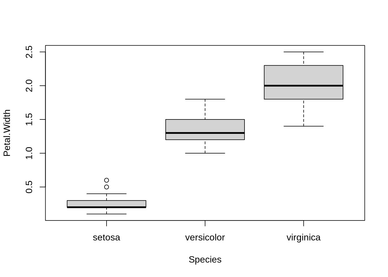

Code

fit=lm(Petal.Width ~ Species, data=iris)
summary(fit)


Call:
lm(formula = Petal.Width ~ Species, data = iris)

Residuals:
   Min     1Q Median     3Q    Max 
-0.626 -0.126 -0.026  0.154  0.474 

Coefficients:
                  Estimate Std. Error t value Pr(>|t|)    
(Intercept)        0.24600    0.02894    8.50 1.96e-14 ***
Speciesversicolor  1.08000    0.04093   26.39  < 2e-16 ***
Speciesvirginica   1.78000    0.04093   43.49  < 2e-16 ***
---
Signif. codes:  0 '***' 0.001 '**' 0.01 '*' 0.05 '.' 0.1 ' ' 1

Residual standard error: 0.2047 on 147 degrees of freedom
Multiple R-squared:  0.9289,    Adjusted R-squared:  0.9279 
F-statistic:   960 on 2 and 147 DF,  p-value: < 2.2e-16

Interpretation:

“setosa” (1st species) has mean Petal.Width=0.246(29) - reference baseline
“versicolor” (2nd species) has mean Petal.Width = Petal.Width(setosa) + 1.08(4)
“virginica” (3rd species) has mean Petal.Width = Petal.Width(setosa) + 1.78(4)

Anova

summary(fit) contains information on the individual coefficients. They are difficult to interpret

Code

anova(fit)

Analysis of Variance Table

Response: Petal.Width
           Df Sum Sq Mean Sq F value    Pr(>F)    
Species     2 80.413  40.207  960.01 < 2.2e-16 ***
Residuals 147  6.157   0.042                      
---
Signif. codes:  0 '***' 0.001 '**' 0.01 '*' 0.05 '.' 0.1 ' ' 1

Interpretation: variable “Species” accounts for much variation in “Petal.Width”

More complicated models

Determine residual standard error sigma for different fits with various complexity

Code

# A list of formulae
formula_list = list(
  Petal.Width ~ Petal.Length,                 # as before (single variable)
  Petal.Width ~ Petal.Length + Sepal.Length,  # function of more than one variable
  Petal.Width ~ Species,                      # function of categorical variables
  Petal.Width ~ .                             # function of all other variable (numerical and categorical)
)

sig=c()
for (f in formula_list) {
  fit = lm(f, data=iris)
  sig = c(sig, sigma(fit))
  print(paste(sigma(fit), format(f)))
}

[1] "0.206484348913609 Petal.Width ~ Petal.Length"
[1] "0.204445704742963 Petal.Width ~ Petal.Length + Sepal.Length"
[1] "0.204650024805914 Petal.Width ~ Species"
[1] "0.166615943019283 Petal.Width ~ ."

Code

# more concise loop using lapply/sapply
# sig = sapply(lapply(formula_list, lm, data=iris), sigma)

op=par(no.readonly=TRUE) 
par(mar=c(4,20,2,2))
barplot(sig ~ format(formula_list), horiz=TRUE, las=2, ylab="", xlab="sigma")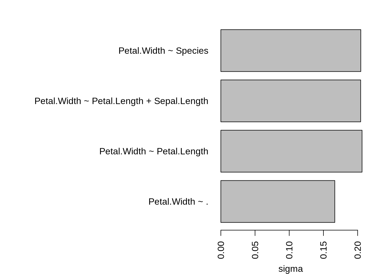

Code

par(op)     # reset graphical parameters

… more complex models tend to have smaller residual standard error (overfitting?)

Model Checking: Diagnostic Plots

“fit” is a large object of the lm-class which contains also lots of diagnostic informmation. Notice how the behaviour of “plot” changes.

Code

fit=lm(Petal.Width ~ ., data=iris)
op=par(no.readonly=TRUE)   # safe only resettable graphical parameters, avoids many warnings
par(mfrow=c(2,2))          # change graphical parameters: 2x2 images on device
plot(fit,col=iris$Species) # four plots rather than one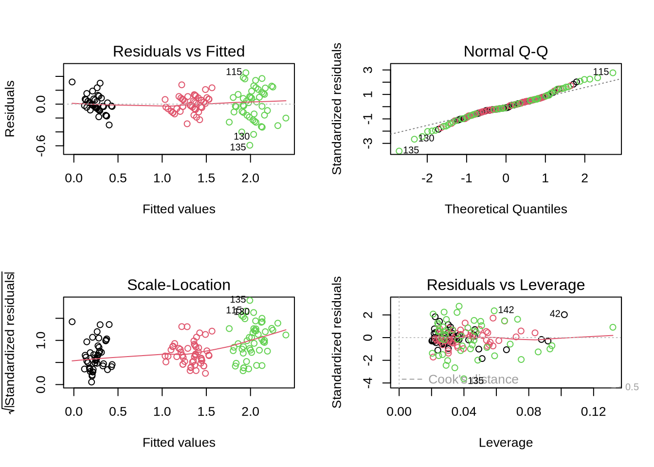

Code

par(op)                    # reset graphical parameters

more examples here: http://www.statmethods.net/stats/regression.html

Linear models \(y_i=\theta_0 + \theta_1 x_i + \epsilon_i\) make certain assumptions (\(\epsilon_i \propto N(0,\sigma^2)\))

residuals \(\epsilon_i\) are independent from each other (non-linear patterns?)
residuals are normally distributed
have equal variance \(\sigma^2\) (“homoscedasticity”)
no outliers (large residuals) or observations with strong influence on fit

Review

dependencies between variable can often be modeled
linear model lm(): fitting, summary and interpretation
linear models with numerical and factorial variables
linear models may not be appropriate \(\to\) example(anscombe)