06: Data Visualization

pheatmap

PCA

Author

Thomas Manke

Goal 1: Show me all the data

Scaling

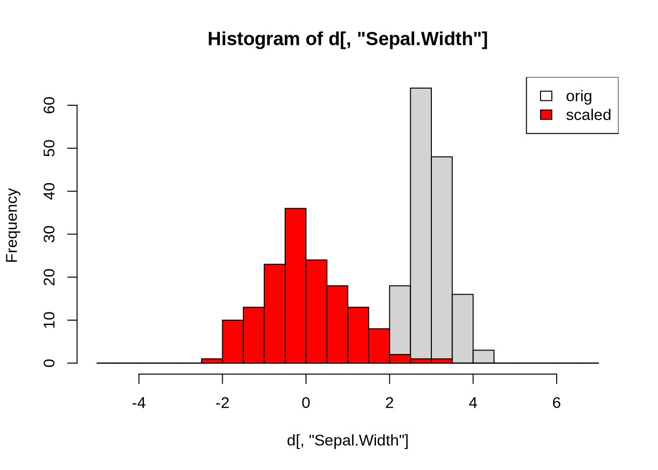
It’s good practice to normalize the different numeric variables

Code

d=iris[,-5]   # numerical iris data (without speciee) 
ds=scale(d)   # scaled iris data (column-wise)

br=seq(-5,7,by=0.5)                                           # set common break points for the histograms below
hist(d[,"Sepal.Width"], breaks = br)                          # illustrate scaling for specific column
hist(ds[,"Sepal.Width"], breaks = br, add=TRUE, col="red")    # add histogram to current plot
legend("topright", c("orig","scaled"), fill=c("white", "red"))

Heatmaps

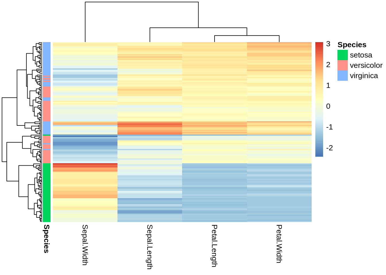
Heatmaps are color-coded representations of numerical matrices.

Typically the rows and columns are re-ordered according to some distance measure (default: Euclidean) and hierarchical clustering method (default: complete)

There are many tools to draw heatmaps in R. Here we use the pheatmap package to provide this powerful functionality

Code

#install.packages("pheatmap")  # That's how we install new packages - more later
library(pheatmap)              # make packaged functions available
paste('loaded pheatmap version:', packageVersion('pheatmap'))

[1] "loaded pheatmap version: 1.0.12"

Code

ds  = scale(iris[,-5])                # scaled data for heatmap
ann = data.frame(Species = iris[,5])  # meta data for annotations

# explicitly set rownames to retain association between data and metadata
rownames(ds)=rownames(iris)
rownames(ann)=rownames(iris)

pheatmap(ds, 
         annotation_row = ann,
         show_rownames = FALSE,
         )

There is many more parameters for more control - if you have lots of time read “?pheatmap”

Sending plots to files

In Rstudio, we can export figures from the “Plots” tab. On the console we can define a pdf file as a new device for all subsequent figures. This is usually done only after the image is sufficiently optimized

Code

pdf("output/heatmap.pdf")                                        # similar for jpeg, png, ...
pheatmap(ds, annotation_row = ann, show_rownames = FALSE)
dev.off()                                                 # close device = pdf file

pdf 
  3

Goal 2: Show me all the data (in lower dimensions)

Code

M=as.matrix(iris[,-5])     # numerical data, some operations below require matrices not data frames (%*%)
s=iris[,5]                 # species attributes (factor)

PCA Goals

simplify description of data matrix $M$: data reduction & extract most important information
maximal variance: look for direction in which data shows maximal variation
minimal error: allow accurate reconstruction of original data

PCA goal from amoeba @ https://stats.stackexchange.com/questions/2691/making-sense-of-principal-component-analysis-eigenvectors-eigenvalues

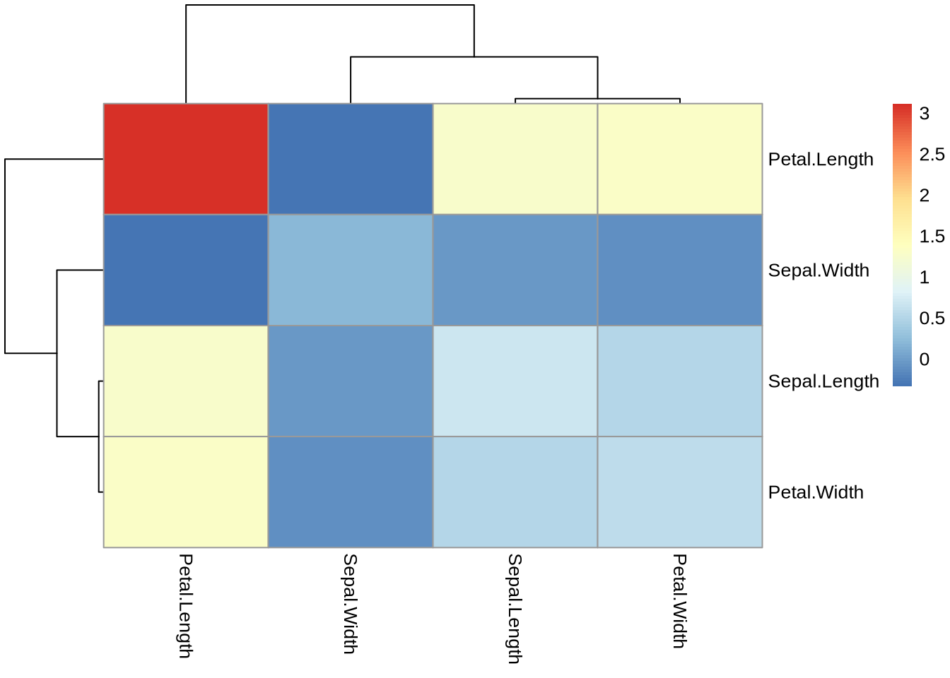
For the iris data, there are many correlations

Code

pheatmap(cor(M)) # original correlation matrix

PCA with R

Code

pca = prcomp(M, scale=TRUE)

Task

What kind of object is pca?

Correlation Structure

Code

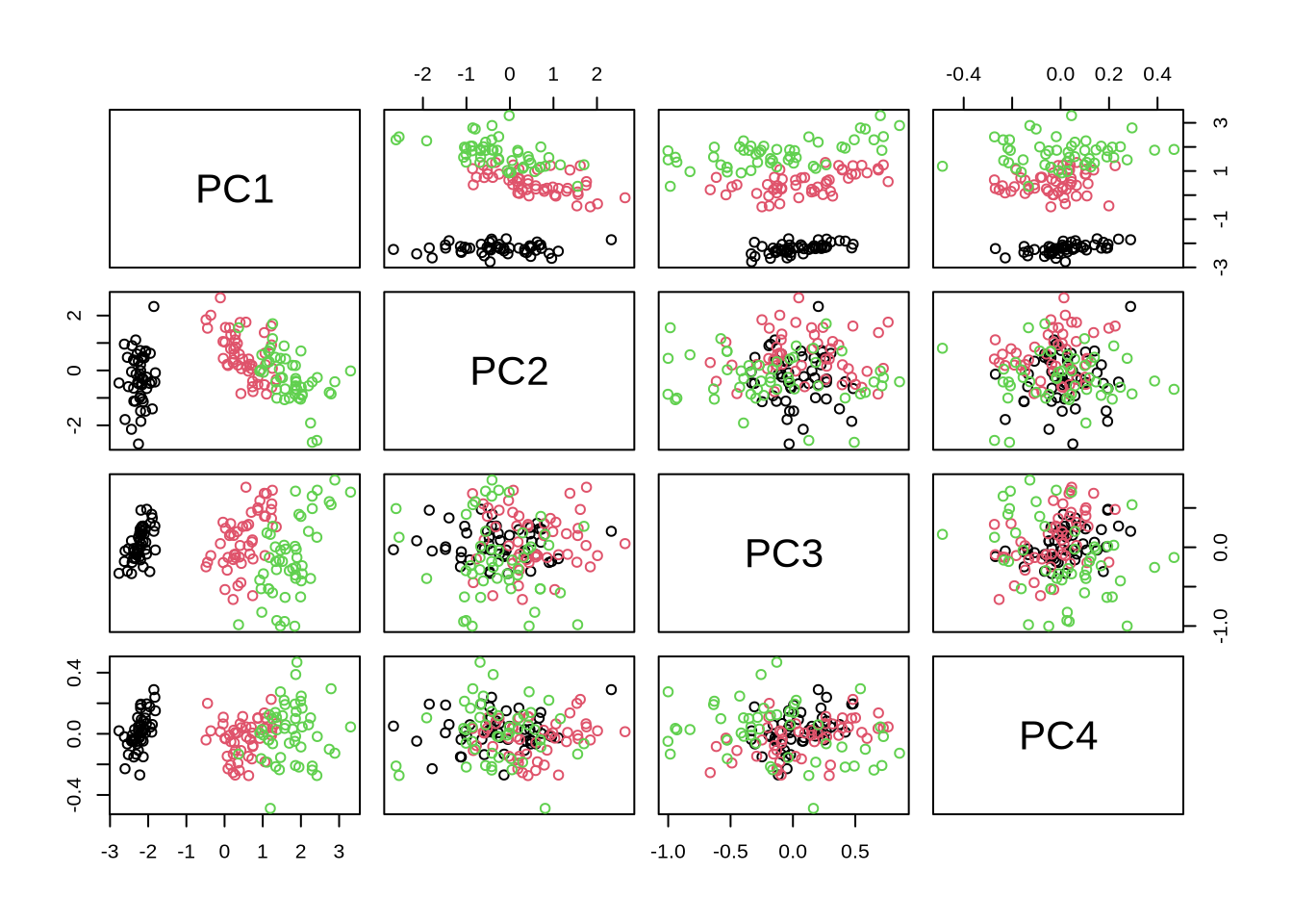
S=pca$x          # score matrix = rotated and scaled data matrix

pairs(S, col=s)

Code

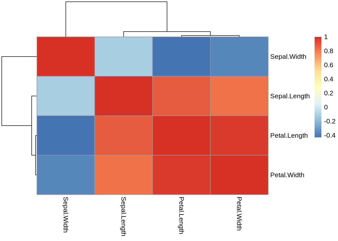
# correlation matrix of scores is diagonal (by design)
# --> principal components are uncorrelated
pheatmap(cor(S))

Ordered Components

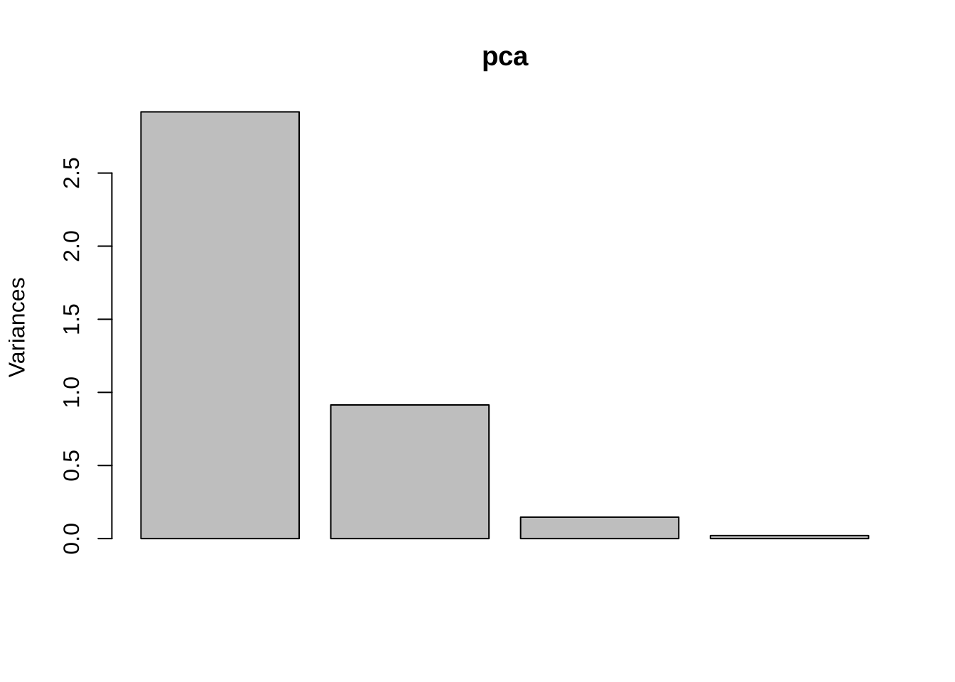
First principle components contribute most to the overall variance

Code

plot(pca)

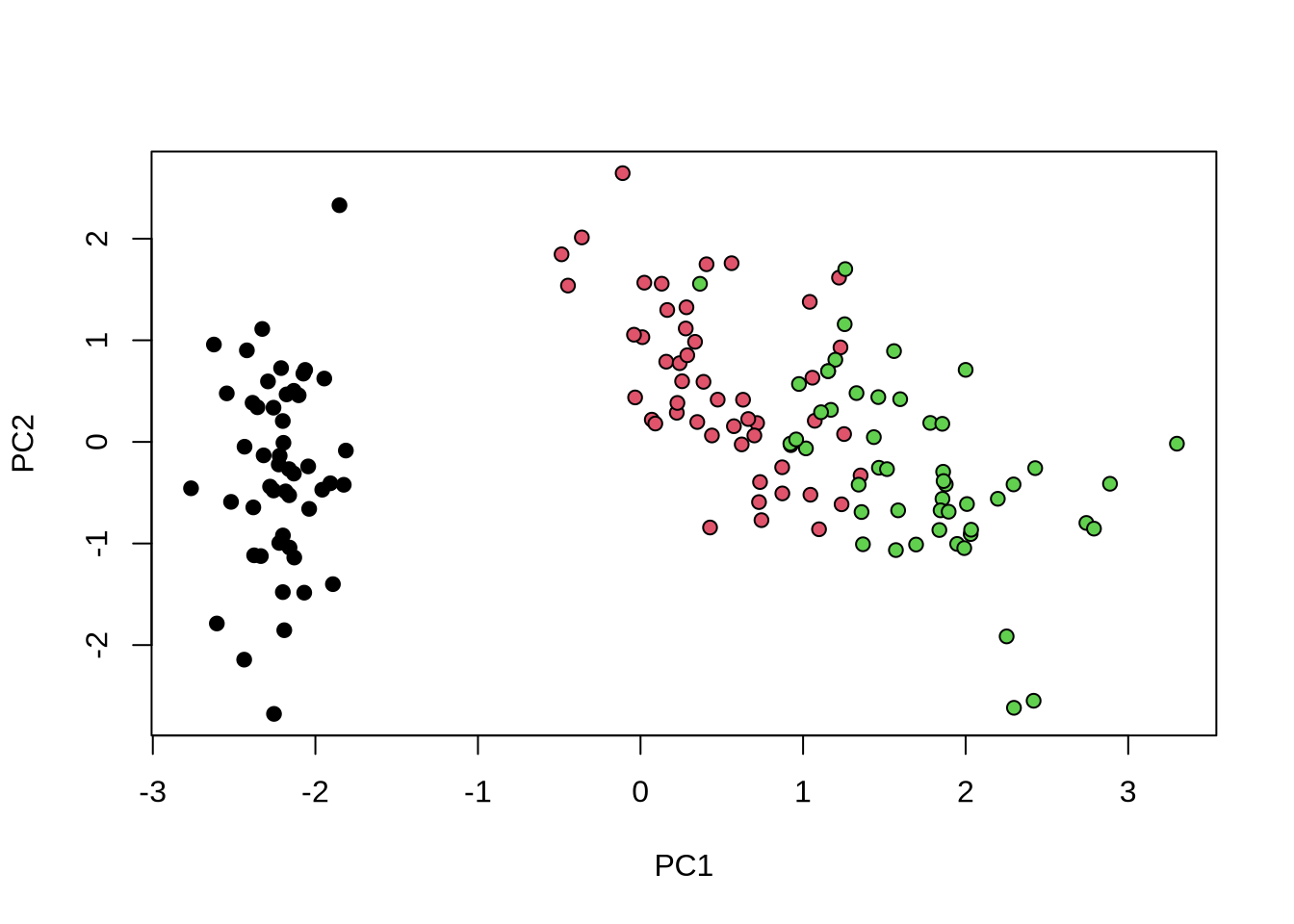
The success of this procedure depends on the data, but if there is a strong ordering, then we might represent the data in only the first two dimensions:

Code

plot(S[,1:2],pch=21, bg=s)  # score-plot

Review

use heatmaps to visualize large matrices
data transformation: scale()
installing packages: pheatmap
exporting figures as publication-ready files: pdf()
dimensional reduction (PCA): prcomp()

--- title: "06: Data Visualization" author: "Thomas Manke" categories: - pheatmap - PCA --- ```{r, child="_setup.qmd"} ``` ## Goal 1: Show me all the data ### Scaling It's good practice to normalize the different numeric variables ```{r scaling} d=iris[,-5] # numerical iris data (without speciee) ds=scale(d) # scaled iris data (column-wise) br=seq(-5,7,by=0.5) # set common break points for the histograms below hist(d[,"Sepal.Width"], breaks = br) # illustrate scaling for specific column hist(ds[,"Sepal.Width"], breaks = br, add=TRUE, col="red") # add histogram to current plot legend("topright", c("orig","scaled"), fill=c("white", "red")) ``` ### Heatmaps Heatmaps are color-coded representations of numerical matrices. Typically the rows and columns are re-ordered according to some distance measure (default: Euclidean) and hierarchical clustering method (default: complete) There are many tools to draw heatmaps in R. Here we use the `pheatmap` package to provide this powerful functionality ```{r pheatmap} #install.packages("pheatmap") # That's how we install new packages - more later library(pheatmap) # make packaged functions available paste('loaded pheatmap version:', packageVersion('pheatmap')) ds = scale(iris[,-5]) # scaled data for heatmap ann = data.frame(Species = iris[,5]) # meta data for annotations # explicitly set rownames to retain association between data and metadata rownames(ds)=rownames(iris) rownames(ann)=rownames(iris) pheatmap(ds, annotation_row = ann, show_rownames = FALSE, ) ``` There is many more parameters for more control - if you have lots of time read "?pheatmap" *** ### Sending plots to files In Rstudio, we can export figures from the "Plots" tab. On the console we can define a pdf file as a new device for all subsequent figures. This is usually done only *after* the image is sufficiently optimized ```{r pdf} pdf("output/heatmap.pdf") # similar for jpeg, png, ... pheatmap(ds, annotation_row = ann, show_rownames = FALSE) dev.off() # close device = pdf file ``` *** ## Goal 2: Show me all the data (in lower dimensions) ```{r df2mat} M=as.matrix(iris[,-5]) # numerical data, some operations below require matrices not data frames (%*%) s=iris[,5] # species attributes (factor) ``` ### PCA Goals * simplify description of data matrix $M$: data reduction & extract most important information * maximal variance: look for direction in which data shows maximal variation * minimal error: allow accurate reconstruction of original data ![PCA goal](images/PCA.gif) from amoeba @ https://stats.stackexchange.com/questions/2691/making-sense-of-principal-component-analysis-eigenvectors-eigenvalues For the iris data, there are many correlations ```{r} pheatmap(cor(M)) # original correlation matrix ``` ### PCA with R ```{r run_pca} pca = prcomp(M, scale=TRUE) ``` #### Task What kind of object is pca? ```{r pca_obj, echo=FALSE, eval=FALSE} class(pca) typeof(pca) str(pca) methods(class="prcomp") ``` ### Correlation Structure ```{r pca_cov} S=pca$x # score matrix = rotated and scaled data matrix pairs(S, col=s) # correlation matrix of scores is diagonal (by design) # --> principal components are uncorrelated pheatmap(cor(S)) ``` ### Ordered Components First principle components contribute most to the overall variance ```{r} plot(pca) ``` The success of this procedure depends on the data, but **if** there is a strong ordering, then we might represent the data in only the **first two dimensions**: ```{r plot_PC1_PC2} plot(S[,1:2],pch=21, bg=s) # score-plot ``` *** ## Review * use heatmaps to visualize large matrices * data transformation: scale() * installing packages: pheatmap * exporting figures as publication-ready files: pdf() * dimensional reduction (PCA): prcomp()