07: Data Import with Tidyverse

Juan Caballero

Before we begin

If you are not using Workbench, please install the following packages:

install.packages("tidyverse")

The command will install a large set of packages that are designed to work together, including ggplot2.

And load the package

library(tidyverse)

Credit

This presentation is heavily influenced by Rafael Irizarry’s book Introduction to Data Science and his corresponding course on EdX.
It also draws on material from previous MPI R courses given by Devon Ryan and David Koppstein.
Updated with the Software Carpentry course “Introduction to data analysis with R and Bioconductor”

Following along

For each module, please create a separate R script and type in and execute the commands that are to follow along.
The code from some slides depends on the previous slides!
You can execute each line individually using Command-Enter on Mac, alt-Enter on Workbench.

Our example dataset

Gender matched eight week old C57BL/6 mice were inoculated saline or with Influenza A (Puerto Rico/8/34; PR8, 1.0 HAU) by intranasal route and transcriptomic changes in the cerebellum and spinal cord tissues were evaluated by RNA-seq (Hiseq-2500 100bp PE-reads) at days 0 (non-infected), 4 and 8.

But for this session, we’ll use https://raw.githubusercontent.com/maxplanck-ie/Rintro/2024.04/qmd/data/rnaseq_counts_wide.csv which contains a table for gene expression (1474 genes) per sample (22 samples)

Data Import in the Tidyverse

The first step for any analysis is importing the data into a machine-readable format. The tidyverse offers the readr:: and readxl:: packages.

Note:

most data can be easy to import when it’s properly formatted in a text format
MS Excel files can be read and/or write but should be avoided

Table formats

CSV (comma separated values)

sample,sex,age,treatment,response
A001,M,8,KO,5200
A002,M,4,WT,4430
A003,F,4,KO,344
B001,F,6,WT,2328

TSV (tab separated values)

sample\tsex\tage\ttreatment\tresponse
A001\tM\t8\tKO\t5200
A002\tM\t4\tWT\t4430
A003\tF\t4\tKO\t344
B001\tF\t6t\tWT\t2328

`readr::`

readr:: is the Tidyverse library for reading data from text formats.
read_csv(), read_tsv(), read_table(), and read_delim() are some of the functions provided
read_csv2() allows for reading of European-style CSV files (e.g. using ;)

`readr::` in action

Example commands, don’t run

# read file in CSV format, file is in working directory
dat = read_csv("file.csv")

# read file using full path, file is anywhere in the filesystem
dat = read_csv("/full/path/to/file.csv")

# read file using URL, file is anywhere in the internet
dat = read_csv("https://server.com/region/file.csv")

`readr::` in action

rna_file = "https://raw.githubusercontent.com/maxplanck-ie/Rintro/2024.04/qmd/data/rnaseq_counts_wide.csv"

rna = read_csv(rna_file)

# What is this "*rna*"?
rna

# A tibble: 1,474 × 23
   gene    GSM2545336 GSM2545337 GSM2545338 GSM2545339 GSM2545340 GSM2545341
   <chr>        <dbl>      <dbl>      <dbl>      <dbl>      <dbl>      <dbl>
 1 Asl           1170        361        400        586        626        988
 2 Apod         36194      10347       9173      10620      13021      29594
 3 Cyp2d22       4060       1616       1603       1901       2171       3349
 4 Klk6           287        629        641        578        448        195
 5 Fcrls           85        233        244        237        180         38
 6 Slc2a4         782        231        248        265        313        786
 7 Exd2          1619       2288       2235       2513       2366       1359
 8 Gjc2           288        595        568        551        310        146
 9 Plp1         43217     101241      96534      58354      53126      27173
10 Gnb4          1071       1791       1867       1430       1355        798
# ℹ 1,464 more rows
# ℹ 16 more variables: GSM2545342 <dbl>, GSM2545343 <dbl>, GSM2545344 <dbl>,
#   GSM2545345 <dbl>, GSM2545346 <dbl>, GSM2545347 <dbl>, GSM2545348 <dbl>,
#   GSM2545349 <dbl>, GSM2545350 <dbl>, GSM2545351 <dbl>, GSM2545352 <dbl>,
#   GSM2545353 <dbl>, GSM2545354 <dbl>, GSM2545362 <dbl>, GSM2545363 <dbl>,
#   GSM2545380 <dbl>

What is a tibble?

Tibbles are like data frames, but more modern, and are built for the Tidyverse
The interface is the same, using e.g. $ for columns
Tibbles can contain more complex objects than just strings, numbers, or booleans, like lists or functions
Tibbles can be grouped
You can see the types of each column in a tibble

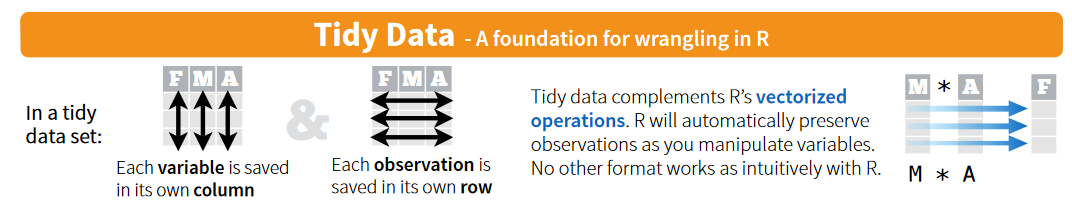
What is Tidy Data?

In tidy data, each row is an observation and each column is a different variable (long-format).
In wide data, each row contains several observations, and the columns contain values (wide-format).

Hands on

Get the basic statistics for each sample in rna

Which sample has the highest mean expression?

Hands on

summary(rna)

     gene             GSM2545336      GSM2545337          GSM2545338   
 Length:1474        Min.   :    0   Min.   :     0.00   Min.   :    0  
 Class :character   1st Qu.:   91   1st Qu.:    56.25   1st Qu.:   52  
 Mode  :character   Median :  611   Median :   494.50   Median :  468  
                    Mean   : 2062   Mean   :  1765.51   Mean   : 1668  
                    3rd Qu.: 2090   3rd Qu.:  1798.75   3rd Qu.: 1692  
                    Max.   :89445   Max.   :101241.00   Max.   :96534  
   GSM2545339         GSM2545340        GSM2545341      GSM2545342     
 Min.   :    0.00   Min.   :    0.0   Min.   :    0   Min.   :    0.0  
 1st Qu.:   77.25   1st Qu.:   59.5   1st Qu.:   47   1st Qu.:   63.0  
 Median :  541.50   Median :  487.0   Median :  462   Median :  470.5  
 Mean   : 1696.12   Mean   : 1681.8   Mean   : 1638   Mean   : 1594.1  
 3rd Qu.: 1772.75   3rd Qu.: 1811.5   3rd Qu.: 1694   3rd Qu.: 1625.8  
 Max.   :58354.00   Max.   :53126.0   Max.   :61758   Max.   :60132.0  
   GSM2545343         GSM2545344        GSM2545345        GSM2545346      
 Min.   :    0.00   Min.   :    0.0   Min.   :    0.0   Min.   :    0.00  
 1st Qu.:   72.25   1st Qu.:   58.0   1st Qu.:   52.0   1st Qu.:   67.25  
 Median :  634.00   Median :  502.5   Median :  497.5   Median :  497.50  
 Mean   : 2106.96   Mean   : 1712.4   Mean   : 1700.2   Mean   : 1692.77  
 3rd Qu.: 2266.25   3rd Qu.: 1778.2   3rd Qu.: 1834.5   3rd Qu.: 1722.25  
 Max.   :98658.00   Max.   :61356.0   Max.   :61647.0   Max.   :71706.00  
   GSM2545347        GSM2545348          GSM2545349      GSM2545350      
 Min.   :    0.0   Min.   :     0.00   Min.   :    0   Min.   :    0.00  
 1st Qu.:   63.0   1st Qu.:    70.25   1st Qu.:   66   1st Qu.:   71.25  
 Median :  549.5   Median :   570.50   Median :  573   Median :  624.00  
 Mean   : 1805.4   Mean   :  1976.72   Mean   : 1871   Mean   : 2208.66  
 3rd Qu.: 1872.0   3rd Qu.:  2038.00   3rd Qu.: 2009   3rd Qu.: 2314.75  
 Max.   :71375.0   Max.   :102790.00   Max.   :82722   Max.   :91642.00  
   GSM2545351        GSM2545352         GSM2545353      GSM2545354   
 Min.   :    0.0   Min.   :    0.00   Min.   :    0   Min.   :    0  
 1st Qu.:   83.0   1st Qu.:   84.25   1st Qu.:   74   1st Qu.:   60  
 Median :  557.5   Median :  647.00   Median :  606   Median :  534  
 Mean   : 1887.7   Mean   : 2181.93   Mean   : 2004   Mean   : 1823  
 3rd Qu.: 1885.2   3rd Qu.: 2294.00   3rd Qu.: 2149   3rd Qu.: 1961  
 Max.   :75277.0   Max.   :74044.00   Max.   :71237   Max.   :84540  
   GSM2545362         GSM2545363      GSM2545380      
 Min.   :    0.00   Min.   :    0   Min.   :    0.00  
 1st Qu.:   93.25   1st Qu.:   48   1st Qu.:   75.25  
 Median :  625.00   Median :  520   Median :  597.50  
 Mean   : 1976.61   Mean   : 1816   Mean   : 2059.77  
 3rd Qu.: 1956.25   3rd Qu.: 1997   3rd Qu.: 2071.25  
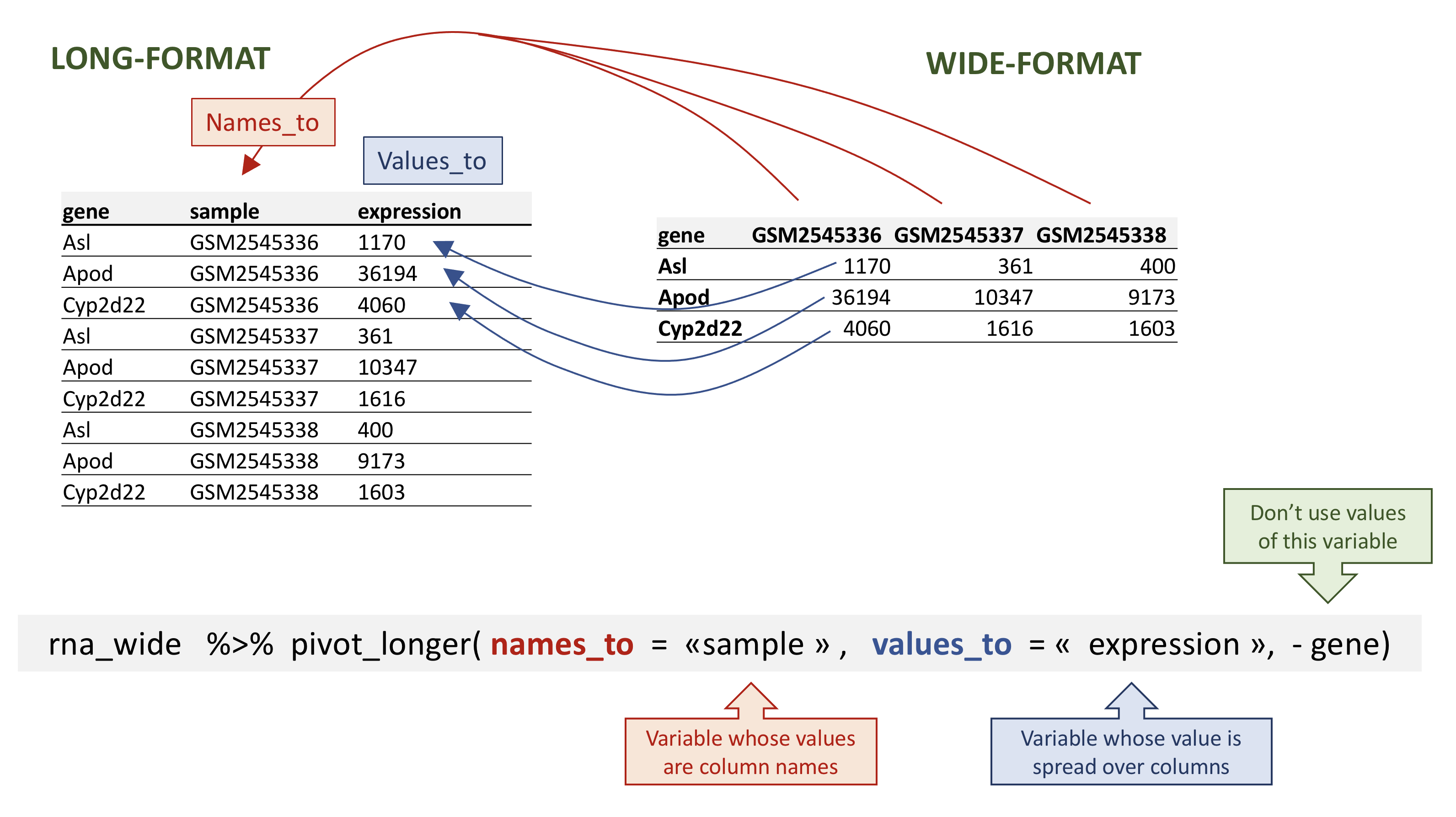
 Max.   :71380.00   Max.   :66033   Max.   :87942.00

Dplyr in action - `pivot_longer()`

To transform the data in a long-format we use pivot_longer(), it takes as inputs:

the data to be transformed;
the names_to the new column name we wish to create and populate with the current column names;
the values_to the new column name we wish to create and populate with current values;
the names of the columns to be used to populate the names_to and values_to variables (or to drop with -).

Dplyr in action - `pivot_longer()`

rna_long = pivot_longer(
                 rna,
                 names_to = "sample",
                 values_to = "expression",
                 -gene)
rna_long

# A tibble: 32,428 × 3
   gene  sample     expression
   <chr> <chr>           <dbl>
 1 Asl   GSM2545336       1170
 2 Asl   GSM2545337        361
 3 Asl   GSM2545338        400
 4 Asl   GSM2545339        586
 5 Asl   GSM2545340        626
 6 Asl   GSM2545341        988
 7 Asl   GSM2545342        836
 8 Asl   GSM2545343        535
 9 Asl   GSM2545344        586
10 Asl   GSM2545345        597
# ℹ 32,418 more rows

Dplyr in action - `pivot_longer()`

Column selection can be defined with patterns

rna_long2 = pivot_longer(
                 rna,
                 names_to = "sample",
                 values_to = "expression",
                 cols = starts_with("GSM"))
rna_long2

# A tibble: 32,428 × 3
   gene  sample     expression
   <chr> <chr>           <dbl>
 1 Asl   GSM2545336       1170
 2 Asl   GSM2545337        361
 3 Asl   GSM2545338        400
 4 Asl   GSM2545339        586
 5 Asl   GSM2545340        626
 6 Asl   GSM2545341        988
 7 Asl   GSM2545342        836
 8 Asl   GSM2545343        535
 9 Asl   GSM2545344        586
10 Asl   GSM2545345        597
# ℹ 32,418 more rows

Dplyr in action - `pivot_longer()`

Column selection can be also defined with ranges

rna_long3 = pivot_longer(
                 rna, 
                 names_to = "sample",
                 values_to = "expression",
                 GSM2545336:GSM2545380)
rna_long3

# A tibble: 32,428 × 3
   gene  sample     expression
   <chr> <chr>           <dbl>
 1 Asl   GSM2545336       1170
 2 Asl   GSM2545337        361
 3 Asl   GSM2545338        400
 4 Asl   GSM2545339        586
 5 Asl   GSM2545340        626
 6 Asl   GSM2545341        988
 7 Asl   GSM2545342        836
 8 Asl   GSM2545343        535
 9 Asl   GSM2545344        586
10 Asl   GSM2545345        597
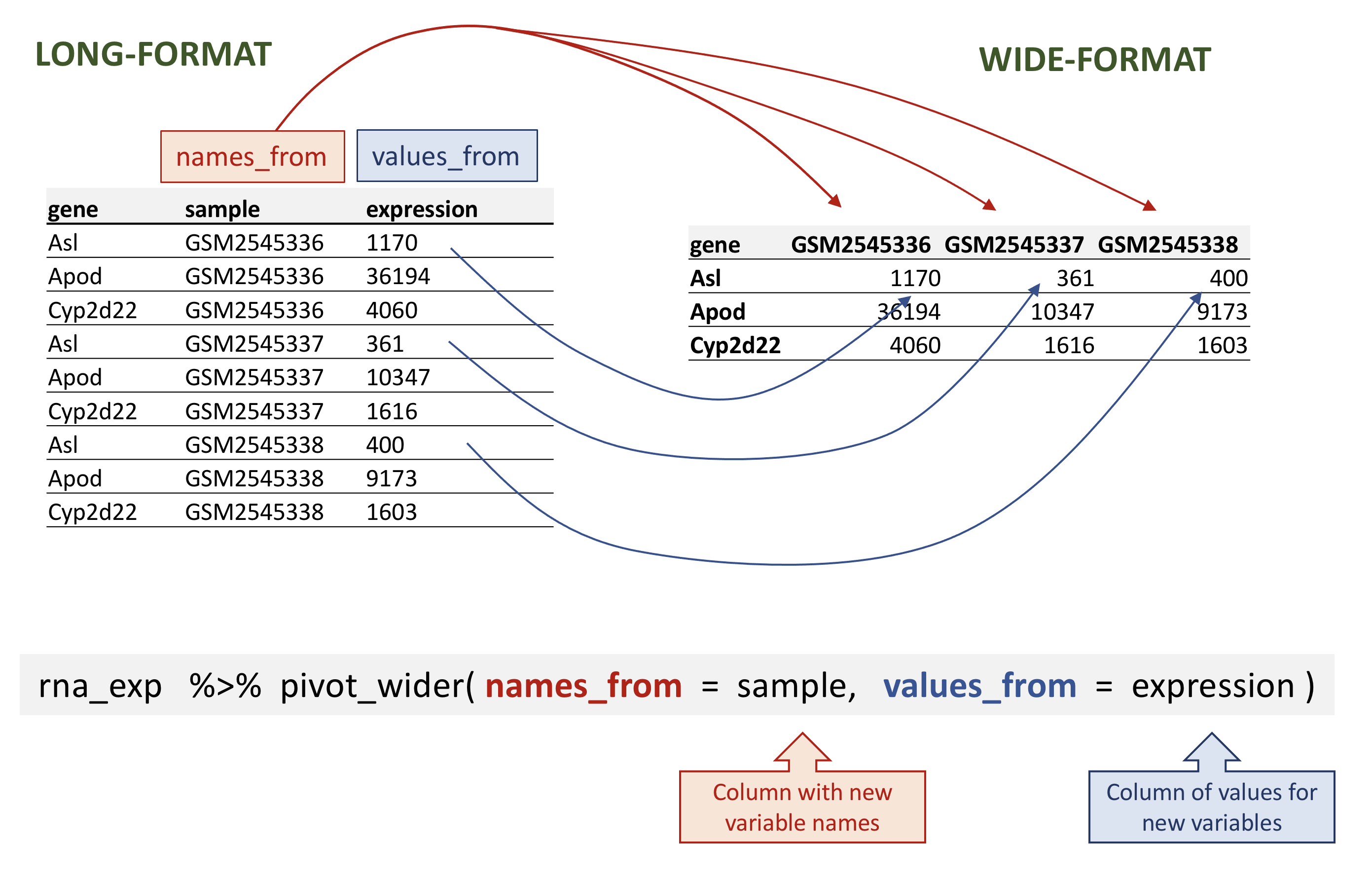
# ℹ 32,418 more rows

Dplyr in action - `pivot_wider()`

The inverse operation is pivot_wider() can transform long-format to wide-format.

It takes three main arguments:

the data to be transformed
the names_from are the column whose values will become new column names
the values_from are the column whose values will fill the new columns

Dplyr in action - `pivot_wider()`

rna_wide = pivot_wider(
                rna_long,
                names_from = sample,
                values_from = expression)
rna_wide

# A tibble: 1,474 × 23
   gene    GSM2545336 GSM2545337 GSM2545338 GSM2545339 GSM2545340 GSM2545341
   <chr>        <dbl>      <dbl>      <dbl>      <dbl>      <dbl>      <dbl>
 1 Asl           1170        361        400        586        626        988
 2 Apod         36194      10347       9173      10620      13021      29594
 3 Cyp2d22       4060       1616       1603       1901       2171       3349
 4 Klk6           287        629        641        578        448        195
 5 Fcrls           85        233        244        237        180         38
 6 Slc2a4         782        231        248        265        313        786
 7 Exd2          1619       2288       2235       2513       2366       1359
 8 Gjc2           288        595        568        551        310        146
 9 Plp1         43217     101241      96534      58354      53126      27173
10 Gnb4          1071       1791       1867       1430       1355        798
# ℹ 1,464 more rows
# ℹ 16 more variables: GSM2545342 <dbl>, GSM2545343 <dbl>, GSM2545344 <dbl>,
#   GSM2545345 <dbl>, GSM2545346 <dbl>, GSM2545347 <dbl>, GSM2545348 <dbl>,
#   GSM2545349 <dbl>, GSM2545350 <dbl>, GSM2545351 <dbl>, GSM2545352 <dbl>,
#   GSM2545353 <dbl>, GSM2545354 <dbl>, GSM2545362 <dbl>, GSM2545363 <dbl>,
#   GSM2545380 <dbl>

Dplyr in action - `pivot_wider()`

By default, missing values will be converted to NA, we can change it with values_fill

rna_wide_noNAs = pivot_wider(
                      rna_long,
                      names_from = sample,
                      values_from = expression,
                      values_fill = 0)
rna_wide_noNAs

# A tibble: 1,474 × 23
   gene    GSM2545336 GSM2545337 GSM2545338 GSM2545339 GSM2545340 GSM2545341
   <chr>        <dbl>      <dbl>      <dbl>      <dbl>      <dbl>      <dbl>
 1 Asl           1170        361        400        586        626        988
 2 Apod         36194      10347       9173      10620      13021      29594
 3 Cyp2d22       4060       1616       1603       1901       2171       3349
 4 Klk6           287        629        641        578        448        195
 5 Fcrls           85        233        244        237        180         38
 6 Slc2a4         782        231        248        265        313        786
 7 Exd2          1619       2288       2235       2513       2366       1359
 8 Gjc2           288        595        568        551        310        146
 9 Plp1         43217     101241      96534      58354      53126      27173
10 Gnb4          1071       1791       1867       1430       1355        798
# ℹ 1,464 more rows
# ℹ 16 more variables: GSM2545342 <dbl>, GSM2545343 <dbl>, GSM2545344 <dbl>,
#   GSM2545345 <dbl>, GSM2545346 <dbl>, GSM2545347 <dbl>, GSM2545348 <dbl>,
#   GSM2545349 <dbl>, GSM2545350 <dbl>, GSM2545351 <dbl>, GSM2545352 <dbl>,
#   GSM2545353 <dbl>, GSM2545354 <dbl>, GSM2545362 <dbl>, GSM2545363 <dbl>,
#   GSM2545380 <dbl>

Dplyr in action - `write_csv`

Finally, we could need to save our data as a new file for later use or sharing, we can use write_csv()

write_csv(rna_wide_noNAs, file = "output/rna_wide.csv")

`readxl::`

readxl:: is the Tidyverse library for reading data from Excel formats
read_excel(), read_xls() and read_xlsx() are some of the functions provided
The excel_sheets() function yields the names of the sheets in the Excel file
But please, don’t use Excel

Any questions?

We will next talk about how to manipulate data in data frames/tibbles using the Tidyverse.

07: Data Import with Tidyverse

Before we begin

Credit

Following along

Our example dataset

Data Import in the Tidyverse

Table formats

readr::

readr:: in action

readr:: in action

What is a tibble?

What is Tidy Data?

Hands on

Hands on

Dplyr in action - pivot_longer()

Dplyr in action - pivot_longer()

Dplyr in action - pivot_longer()

Dplyr in action - pivot_longer()

Dplyr in action - pivot_longer()

Dplyr in action - pivot_wider()

Dplyr in action - pivot_wider()

Dplyr in action - pivot_wider()

Dplyr in action - pivot_wider()

Dplyr in action - write_csv

readxl::

Any questions?

`readr::`

`readr::` in action

`readr::` in action

Dplyr in action - `pivot_longer()`

Dplyr in action - `pivot_longer()`

Dplyr in action - `pivot_longer()`

Dplyr in action - `pivot_longer()`

Dplyr in action - `pivot_longer()`

Dplyr in action - `pivot_wider()`

Dplyr in action - `pivot_wider()`

Dplyr in action - `pivot_wider()`

Dplyr in action - `pivot_wider()`

Dplyr in action - `write_csv`

`readxl::`