08: Intro to Data Wrangling with Dplyr
Introduction to Dplyr
Dplyr uses a functions that act as verbs to transform data frames in ways to facilitate data analysis.
The six main verbs are:
mutate(): creates new columnsfilter(): filters rows based on criteriaselect(): selects columnssummarize(): creates summary statisticsgroup_by(): analysis on subsets based on a columnarrange(): sorts rows
Dplyr in action
rnaseq.csv is the long-format for the mouse influenza experiment.
Dplyr in action
Contains: gene, sample, expression, organism, age, sex, infection, strain, time, tissue, mouse, ENTREZID, product, ensembl_gene_id, external_synonym, chromosome_name, gene_biotype, phenotype_description, hsapiens_homolog_associated_gene_name
# A tibble: 32,428 × 19
   gene    sample  expression organism   age sex   infection strain  time tissue
   <chr>   <chr>        <dbl> <chr>    <dbl> <chr> <chr>     <chr>  <dbl> <chr>
 1 Asl     GSM254…       1170 Mus mus…     8 Fema… Influenz… C57BL…     8 Cereb…
 2 Apod    GSM254…      36194 Mus mus…     8 Fema… Influenz… C57BL…     8 Cereb…
 3 Cyp2d22 GSM254…       4060 Mus mus…     8 Fema… Influenz… C57BL…     8 Cereb…
 4 Klk6    GSM254…        287 Mus mus…     8 Fema… Influenz… C57BL…     8 Cereb…
 5 Fcrls   GSM254…         85 Mus mus…     8 Fema… Influenz… C57BL…     8 Cereb…
 6 Slc2a4  GSM254…        782 Mus mus…     8 Fema… Influenz… C57BL…     8 Cereb…
 7 Exd2    GSM254…       1619 Mus mus…     8 Fema… Influenz… C57BL…     8 Cereb…
 8 Gjc2    GSM254…        288 Mus mus…     8 Fema… Influenz… C57BL…     8 Cereb…
 9 Plp1    GSM254…      43217 Mus mus…     8 Fema… Influenz… C57BL…     8 Cereb…
10 Gnb4    GSM254…       1071 Mus mus…     8 Fema… Influenz… C57BL…     8 Cereb…
# ℹ 32,418 more rows
# ℹ 9 more variables: mouse <dbl>, ENTREZID <dbl>, product <chr>,
#   ensembl_gene_id <chr>, external_synonym <chr>, chromosome_name <chr>,
#   gene_biotype <chr>, phenotype_description <chr>,
#   hsapiens_homolog_associated_gene_name <chr>
Dplyr in action - select()
Syntax: select(data, col1, col2, col3, ...)
# A tibble: 32,428 × 4
   gene    sample     tissue     expression
   <chr>   <chr>      <chr>           <dbl>
 1 Asl     GSM2545336 Cerebellum       1170
 2 Apod    GSM2545336 Cerebellum      36194
 3 Cyp2d22 GSM2545336 Cerebellum       4060
 4 Klk6    GSM2545336 Cerebellum        287
 5 Fcrls   GSM2545336 Cerebellum         85
 6 Slc2a4  GSM2545336 Cerebellum        782
 7 Exd2    GSM2545336 Cerebellum       1619
 8 Gjc2    GSM2545336 Cerebellum        288
 9 Plp1    GSM2545336 Cerebellum      43217
10 Gnb4    GSM2545336 Cerebellum       1071
# ℹ 32,418 more rows
Dplyr in action - select()
Column exclusion can be defined with -
Hands on
Select
gene, ensembl_gene_id, hsapiens_homolog_associated_gene_nameSelect
gene, gene_biotype, phenotype_description
Hands on
- Select
gene, ensembl_gene_id, hsapiens_homolog_associated_gene_name
# A tibble: 32,428 × 3
   gene    ensembl_gene_id    hsapiens_homolog_associated_gene_name
   <chr>   <chr>              <chr>
 1 Asl     ENSMUSG00000025533 ASL
 2 Apod    ENSMUSG00000022548 APOD
 3 Cyp2d22 ENSMUSG00000061740 CYP2D6
 4 Klk6    ENSMUSG00000050063 KLK6
 5 Fcrls   ENSMUSG00000015852 FCRL2
 6 Slc2a4  ENSMUSG00000018566 SLC2A4
 7 Exd2    ENSMUSG00000032705 EXD2
 8 Gjc2    ENSMUSG00000043448 GJC2
 9 Plp1    ENSMUSG00000031425 PLP1
10 Gnb4    ENSMUSG00000027669 GNB4
# ℹ 32,418 more rows
Hands on
- Select
gene, gene_biotype, phenotype_description
# A tibble: 32,428 × 3
   gene    gene_biotype   phenotype_description
   <chr>   <chr>          <chr>
 1 Asl     protein_coding abnormal circulating amino acid level
 2 Apod    protein_coding abnormal lipid homeostasis
 3 Cyp2d22 protein_coding abnormal skin morphology
 4 Klk6    protein_coding abnormal cytokine level
 5 Fcrls   protein_coding decreased CD8-positive alpha-beta T cell number
 6 Slc2a4  protein_coding abnormal circulating glucose level
 7 Exd2    protein_coding <NA>
 8 Gjc2    protein_coding Purkinje cell degeneration
 9 Plp1    protein_coding abnormal CNS glial cell morphology
10 Gnb4    protein_coding decreased anxiety-related response
# ℹ 32,418 more rows
Dplyr in action - filter()
Syntax: filter(data, filters)
Comparisons: == > >= < <=
# A tibble: 14,740 × 19
   gene    sample  expression organism   age sex   infection strain  time tissue
   <chr>   <chr>        <dbl> <chr>    <dbl> <chr> <chr>     <chr>  <dbl> <chr>
 1 Asl     GSM254…        626 Mus mus…     8 Male  Influenz… C57BL…     4 Cereb…
 2 Apod    GSM254…      13021 Mus mus…     8 Male  Influenz… C57BL…     4 Cereb…
 3 Cyp2d22 GSM254…       2171 Mus mus…     8 Male  Influenz… C57BL…     4 Cereb…
 4 Klk6    GSM254…        448 Mus mus…     8 Male  Influenz… C57BL…     4 Cereb…
 5 Fcrls   GSM254…        180 Mus mus…     8 Male  Influenz… C57BL…     4 Cereb…
 6 Slc2a4  GSM254…        313 Mus mus…     8 Male  Influenz… C57BL…     4 Cereb…
 7 Exd2    GSM254…       2366 Mus mus…     8 Male  Influenz… C57BL…     4 Cereb…
 8 Gjc2    GSM254…        310 Mus mus…     8 Male  Influenz… C57BL…     4 Cereb…
 9 Plp1    GSM254…      53126 Mus mus…     8 Male  Influenz… C57BL…     4 Cereb…
10 Gnb4    GSM254…       1355 Mus mus…     8 Male  Influenz… C57BL…     4 Cereb…
# ℹ 14,730 more rows
# ℹ 9 more variables: mouse <dbl>, ENTREZID <dbl>, product <chr>,
#   ensembl_gene_id <chr>, external_synonym <chr>, chromosome_name <chr>,
#   gene_biotype <chr>, phenotype_description <chr>,
#   hsapiens_homolog_associated_gene_name <chr>
Dplyr in action - filter()
Logical operators: & | ! xor()
# get data which sex is Male AND infection status is NonInfected
filter(rna, sex == "Male" & infection == "NonInfected")
# A tibble: 4,422 × 19
gene sample expression organism age sex infection strain time tissue
<chr> <chr> <dbl> <chr> <dbl> <chr> <chr> <chr> <dbl> <chr>
1 Asl GSM254… 535 Mus mus… 8 Male NonInfec… C57BL… 0 Cereb…
2 Apod GSM254… 13668 Mus mus… 8 Male NonInfec… C57BL… 0 Cereb…
3 Cyp2d22 GSM254… 2008 Mus mus… 8 Male NonInfec… C57BL… 0 Cereb…
4 Klk6 GSM254… 1101 Mus mus… 8 Male NonInfec… C57BL… 0 Cereb…
5 Fcrls GSM254… 375 Mus mus… 8 Male NonInfec… C57BL… 0 Cereb…
6 Slc2a4 GSM254… 249 Mus mus… 8 Male NonInfec… C57BL… 0 Cereb…
7 Exd2 GSM254… 3126 Mus mus… 8 Male NonInfec… C57BL… 0 Cereb…
8 Gjc2 GSM254… 791 Mus mus… 8 Male NonInfec… C57BL… 0 Cereb…
9 Plp1 GSM254… 98658 Mus mus… 8 Male NonInfec… C57BL… 0 Cereb…
10 Gnb4 GSM254… 2437 Mus mus… 8 Male NonInfec… C57BL… 0 Cereb…
# ℹ 4,412 more rows
# ℹ 9 more variables: mouse <dbl>, ENTREZID <dbl>, product <chr>,
# ensembl_gene_id <chr>, external_synonym <chr>, chromosome_name <chr>,
# gene_biotype <chr>, phenotype_description <chr>,
# hsapiens_homolog_associated_gene_name <chr>Dplyr in action - filter()
Multiple filters can be used with ,
# get data which sex is Male AND infection status is NonInfected
filter(rna, sex == "Male", infection == "NonInfected")
# A tibble: 4,422 × 19
gene sample expression organism age sex infection strain time tissue
<chr> <chr> <dbl> <chr> <dbl> <chr> <chr> <chr> <dbl> <chr>
1 Asl GSM254… 535 Mus mus… 8 Male NonInfec… C57BL… 0 Cereb…
2 Apod GSM254… 13668 Mus mus… 8 Male NonInfec… C57BL… 0 Cereb…
3 Cyp2d22 GSM254… 2008 Mus mus… 8 Male NonInfec… C57BL… 0 Cereb…
4 Klk6 GSM254… 1101 Mus mus… 8 Male NonInfec… C57BL… 0 Cereb…
5 Fcrls GSM254… 375 Mus mus… 8 Male NonInfec… C57BL… 0 Cereb…
6 Slc2a4 GSM254… 249 Mus mus… 8 Male NonInfec… C57BL… 0 Cereb…
7 Exd2 GSM254… 3126 Mus mus… 8 Male NonInfec… C57BL… 0 Cereb…
8 Gjc2 GSM254… 791 Mus mus… 8 Male NonInfec… C57BL… 0 Cereb…
9 Plp1 GSM254… 98658 Mus mus… 8 Male NonInfec… C57BL… 0 Cereb…
10 Gnb4 GSM254… 2437 Mus mus… 8 Male NonInfec… C57BL… 0 Cereb…
# ℹ 4,412 more rows
# ℹ 9 more variables: mouse <dbl>, ENTREZID <dbl>, product <chr>,
# ensembl_gene_id <chr>, external_synonym <chr>, chromosome_name <chr>,
# gene_biotype <chr>, phenotype_description <chr>,
# hsapiens_homolog_associated_gene_name <chr>Hands on
Filter data for
femalesandinfectedFilter data for
Cerebellumintime 0
Hands on
- Filter data for
femalesandinfected
# A tibble: 11,792 × 19
   gene    sample  expression organism   age sex   infection strain  time tissue
   <chr>   <chr>        <dbl> <chr>    <dbl> <chr> <chr>     <chr>  <dbl> <chr>
 1 Asl     GSM254…       1170 Mus mus…     8 Fema… Influenz… C57BL…     8 Cereb…
 2 Apod    GSM254…      36194 Mus mus…     8 Fema… Influenz… C57BL…     8 Cereb…
 3 Cyp2d22 GSM254…       4060 Mus mus…     8 Fema… Influenz… C57BL…     8 Cereb…
 4 Klk6    GSM254…        287 Mus mus…     8 Fema… Influenz… C57BL…     8 Cereb…
 5 Fcrls   GSM254…         85 Mus mus…     8 Fema… Influenz… C57BL…     8 Cereb…
 6 Slc2a4  GSM254…        782 Mus mus…     8 Fema… Influenz… C57BL…     8 Cereb…
 7 Exd2    GSM254…       1619 Mus mus…     8 Fema… Influenz… C57BL…     8 Cereb…
 8 Gjc2    GSM254…        288 Mus mus…     8 Fema… Influenz… C57BL…     8 Cereb…
 9 Plp1    GSM254…      43217 Mus mus…     8 Fema… Influenz… C57BL…     8 Cereb…
10 Gnb4    GSM254…       1071 Mus mus…     8 Fema… Influenz… C57BL…     8 Cereb…
# ℹ 11,782 more rows
# ℹ 9 more variables: mouse <dbl>, ENTREZID <dbl>, product <chr>,
#   ensembl_gene_id <chr>, external_synonym <chr>, chromosome_name <chr>,
#   gene_biotype <chr>, phenotype_description <chr>,
#   hsapiens_homolog_associated_gene_name <chr>
Hands on
- Filter data for
Cerebellumintime 0
# A tibble: 10,318 × 19
   gene    sample  expression organism   age sex   infection strain  time tissue
   <chr>   <chr>        <dbl> <chr>    <dbl> <chr> <chr>     <chr>  <dbl> <chr>
 1 Asl     GSM254…        361 Mus mus…     8 Fema… NonInfec… C57BL…     0 Cereb…
 2 Apod    GSM254…      10347 Mus mus…     8 Fema… NonInfec… C57BL…     0 Cereb…
 3 Cyp2d22 GSM254…       1616 Mus mus…     8 Fema… NonInfec… C57BL…     0 Cereb…
 4 Klk6    GSM254…        629 Mus mus…     8 Fema… NonInfec… C57BL…     0 Cereb…
 5 Fcrls   GSM254…        233 Mus mus…     8 Fema… NonInfec… C57BL…     0 Cereb…
 6 Slc2a4  GSM254…        231 Mus mus…     8 Fema… NonInfec… C57BL…     0 Cereb…
 7 Exd2    GSM254…       2288 Mus mus…     8 Fema… NonInfec… C57BL…     0 Cereb…
 8 Gjc2    GSM254…        595 Mus mus…     8 Fema… NonInfec… C57BL…     0 Cereb…
 9 Plp1    GSM254…     101241 Mus mus…     8 Fema… NonInfec… C57BL…     0 Cereb…
10 Gnb4    GSM254…       1791 Mus mus…     8 Fema… NonInfec… C57BL…     0 Cereb…
# ℹ 10,308 more rows
# ℹ 9 more variables: mouse <dbl>, ENTREZID <dbl>, product <chr>,
#   ensembl_gene_id <chr>, external_synonym <chr>, chromosome_name <chr>,
#   gene_biotype <chr>, phenotype_description <chr>,
#   hsapiens_homolog_associated_gene_name <chr>
Dplyr in action - filter()
It can evaluate missing values with is.na()
# get data which human ortholog gene is not defined (*NA*)
filter(rna, is.na(hsapiens_homolog_associated_gene_name))
# A tibble: 4,290 × 19
gene sample expression organism age sex infection strain time tissue
<chr> <chr> <dbl> <chr> <dbl> <chr> <chr> <chr> <dbl> <chr>
1 Prodh GSM25… 2385 Mus mus… 8 Fema… Influenz… C57BL… 8 Cereb…
2 Tssk5 GSM25… 368 Mus mus… 8 Fema… Influenz… C57BL… 8 Cereb…
3 Vmn2r1 GSM25… 116 Mus mus… 8 Fema… Influenz… C57BL… 8 Cereb…
4 Gm10654 GSM25… 472 Mus mus… 8 Fema… Influenz… C57BL… 8 Cereb…
5 Hexa GSM25… 1208 Mus mus… 8 Fema… Influenz… C57BL… 8 Cereb…
6 Sult1a1 GSM25… 1658 Mus mus… 8 Fema… Influenz… C57BL… 8 Cereb…
7 Gm6277 GSM25… 134 Mus mus… 8 Fema… Influenz… C57BL… 8 Cereb…
8 Tmem198b GSM25… 689 Mus mus… 8 Fema… Influenz… C57BL… 8 Cereb…
9 Adam1a GSM25… 440 Mus mus… 8 Fema… Influenz… C57BL… 8 Cereb…
10 Ebp GSM25… 798 Mus mus… 8 Fema… Influenz… C57BL… 8 Cereb…
# ℹ 4,280 more rows
# ℹ 9 more variables: mouse <dbl>, ENTREZID <dbl>, product <chr>,
# ensembl_gene_id <chr>, external_synonym <chr>, chromosome_name <chr>,
# gene_biotype <chr>, phenotype_description <chr>,
# hsapiens_homolog_associated_gene_name <chr>Dplyr in action - filter()
# get data which human ortholog gene is defined (not *NA*)
filter(rna, !is.na(hsapiens_homolog_associated_gene_name))
# A tibble: 28,138 × 19
gene sample expression organism age sex infection strain time tissue
<chr> <chr> <dbl> <chr> <dbl> <chr> <chr> <chr> <dbl> <chr>
1 Asl GSM254… 1170 Mus mus… 8 Fema… Influenz… C57BL… 8 Cereb…
2 Apod GSM254… 36194 Mus mus… 8 Fema… Influenz… C57BL… 8 Cereb…
3 Cyp2d22 GSM254… 4060 Mus mus… 8 Fema… Influenz… C57BL… 8 Cereb…
4 Klk6 GSM254… 287 Mus mus… 8 Fema… Influenz… C57BL… 8 Cereb…
5 Fcrls GSM254… 85 Mus mus… 8 Fema… Influenz… C57BL… 8 Cereb…
6 Slc2a4 GSM254… 782 Mus mus… 8 Fema… Influenz… C57BL… 8 Cereb…
7 Exd2 GSM254… 1619 Mus mus… 8 Fema… Influenz… C57BL… 8 Cereb…
8 Gjc2 GSM254… 288 Mus mus… 8 Fema… Influenz… C57BL… 8 Cereb…
9 Plp1 GSM254… 43217 Mus mus… 8 Fema… Influenz… C57BL… 8 Cereb…
10 Gnb4 GSM254… 1071 Mus mus… 8 Fema… Influenz… C57BL… 8 Cereb…
# ℹ 28,128 more rows
# ℹ 9 more variables: mouse <dbl>, ENTREZID <dbl>, product <chr>,
# ensembl_gene_id <chr>, external_synonym <chr>, chromosome_name <chr>,
# gene_biotype <chr>, phenotype_description <chr>,
# hsapiens_homolog_associated_gene_name <chr>Dplyr in action - Pipes
What if you want to select and filter?
For example get gene, sample, tissue, expression for Males
Option 1. Generate intermediate tables
Option 2. Use nested operations
Option 3. Plumbering with Pipes
Dplyr in action - Pipes
Option 1. Generate intermediate tables
Why is this bad?
Dplyr in action - Pipes
Option 2. Use nested operations
Why is this also bad?
Dplyr in action - Pipes
Option 3. Plumbering with Pipes - Yeah!
Pipes in R look like %>% (made available via the magrittr package) or |> (through base R)
Is this better?
# A tibble: 14,740 × 4
   gene    sample     tissue     expression
   <chr>   <chr>      <chr>           <dbl>
 1 Asl     GSM2545340 Cerebellum        626
 2 Apod    GSM2545340 Cerebellum      13021
 3 Cyp2d22 GSM2545340 Cerebellum       2171
 4 Klk6    GSM2545340 Cerebellum        448
 5 Fcrls   GSM2545340 Cerebellum        180
 6 Slc2a4  GSM2545340 Cerebellum        313
 7 Exd2    GSM2545340 Cerebellum       2366
 8 Gjc2    GSM2545340 Cerebellum        310
 9 Plp1    GSM2545340 Cerebellum      53126
10 Gnb4    GSM2545340 Cerebellum       1355
# ℹ 14,730 more rows
Hands on
Using pipes, subset the rna data to keep observations in female mice at time 0, where the gene has an expression higher than 50000, and retain only the columns gene, sample, time, expression and age.
Hands on
Solution
rna %>%
  filter(expression > 50000, sex == "Female", time == 0 ) %>%
  select(gene, sample, time, expression, sex)
# A tibble: 9 × 5
gene sample time expression sex
<chr> <chr> <dbl> <dbl> <chr>
1 Plp1 GSM2545337 0 101241 Female
2 Atp1b1 GSM2545337 0 53260 Female
3 Plp1 GSM2545338 0 96534 Female
4 Atp1b1 GSM2545338 0 50614 Female
5 Plp1 GSM2545348 0 102790 Female
6 Atp1b1 GSM2545348 0 59544 Female
7 Plp1 GSM2545353 0 71237 Female
8 Glul GSM2545353 0 52451 Female
9 Atp1b1 GSM2545353 0 61451 FemaleDplyr in action - mutate()
As frequently we want to add new columns based on existing data, we can expand the tibble with mutate().
In our example, time is defined in days, let’s add a new column for time in hours (time_hours)
Dplyr in action - mutate()
The new columns can be used to generate another columns, for example, adding a time in minutes based on time in hours:
rna %>%
  mutate(time_hours = time * 24,
         time_min = time_hours * 60) %>%
  select(time, time_hours, time_min)
# A tibble: 32,428 × 3
time time_hours time_min
<dbl> <dbl> <dbl>
1 8 192 11520
2 8 192 11520
3 8 192 11520
4 8 192 11520
5 8 192 11520
6 8 192 11520
7 8 192 11520
8 8 192 11520
9 8 192 11520
10 8 192 11520
# ℹ 32,418 more rowsHands on
Create a new data frame from the rna data that meets the following criteria: contains only gene, chromosome_name, phenotype_description, sample, expression. The expression values should be log-transformed. This data must only contain genes located on sex chromosomes, associated with a phenotype_description, and with a log-expression higher than 5.
Hint: think about how the commands should be ordered to produce this!
Hands on
Solution:
rna %>%
  filter(chromosome_name == "X" | chromosome_name == "Y") %>%
  filter(!is.na(phenotype_description)) %>%
  mutate(expression_log = log(expression)) %>%
  select(gene, chromosome_name, phenotype_description, sample, expression_log) %>%
  filter(expression_log > 5)
# A tibble: 649 × 5
gene chromosome_name phenotype_description sample expression_log
<chr> <chr> <chr> <chr> <dbl>
1 Plp1 X abnormal CNS glial cell morphol… GSM25… 10.7
2 Slc7a3 X decreased body length GSM25… 5.46
3 Plxnb3 X abnormal coat appearance GSM25… 6.58
4 Rbm3 X abnormal liver morphology GSM25… 9.32
5 Cfp X abnormal cardiovascular system … GSM25… 6.18
6 Ebp X abnormal embryonic erythrocyte … GSM25… 6.68
7 Cd99l2 X abnormal cellular extravasation GSM25… 8.04
8 Piga X abnormal brain development GSM25… 6.06
9 Pim2 X decreased T cell proliferation GSM25… 7.11
10 Itm2a X no abnormal phenotype detected GSM25… 7.48
# ℹ 639 more rowsDplyr in action - group_by()
Data analysis commonly needs to split the data, perfom computations and then combine the results (split-apply-combine paradigm)
# A tibble: 32,428 × 19
# Groups:   gene [1,474]
   gene    sample  expression organism   age sex   infection strain  time tissue
   <chr>   <chr>        <dbl> <chr>    <dbl> <chr> <chr>     <chr>  <dbl> <chr>
 1 Asl     GSM254…       1170 Mus mus…     8 Fema… Influenz… C57BL…     8 Cereb…
 2 Apod    GSM254…      36194 Mus mus…     8 Fema… Influenz… C57BL…     8 Cereb…
 3 Cyp2d22 GSM254…       4060 Mus mus…     8 Fema… Influenz… C57BL…     8 Cereb…
 4 Klk6    GSM254…        287 Mus mus…     8 Fema… Influenz… C57BL…     8 Cereb…
 5 Fcrls   GSM254…         85 Mus mus…     8 Fema… Influenz… C57BL…     8 Cereb…
 6 Slc2a4  GSM254…        782 Mus mus…     8 Fema… Influenz… C57BL…     8 Cereb…
 7 Exd2    GSM254…       1619 Mus mus…     8 Fema… Influenz… C57BL…     8 Cereb…
 8 Gjc2    GSM254…        288 Mus mus…     8 Fema… Influenz… C57BL…     8 Cereb…
 9 Plp1    GSM254…      43217 Mus mus…     8 Fema… Influenz… C57BL…     8 Cereb…
10 Gnb4    GSM254…       1071 Mus mus…     8 Fema… Influenz… C57BL…     8 Cereb…
# ℹ 32,418 more rows
# ℹ 9 more variables: mouse <dbl>, ENTREZID <dbl>, product <chr>,
#   ensembl_gene_id <chr>, external_synonym <chr>, chromosome_name <chr>,
#   gene_biotype <chr>, phenotype_description <chr>,
#   hsapiens_homolog_associated_gene_name <chr>
Dplyr in action - group_by()
# A tibble: 32,428 × 19
# Groups:   sample [22]
   gene    sample  expression organism   age sex   infection strain  time tissue
   <chr>   <chr>        <dbl> <chr>    <dbl> <chr> <chr>     <chr>  <dbl> <chr>
 1 Asl     GSM254…       1170 Mus mus…     8 Fema… Influenz… C57BL…     8 Cereb…
 2 Apod    GSM254…      36194 Mus mus…     8 Fema… Influenz… C57BL…     8 Cereb…
 3 Cyp2d22 GSM254…       4060 Mus mus…     8 Fema… Influenz… C57BL…     8 Cereb…
 4 Klk6    GSM254…        287 Mus mus…     8 Fema… Influenz… C57BL…     8 Cereb…
 5 Fcrls   GSM254…         85 Mus mus…     8 Fema… Influenz… C57BL…     8 Cereb…
 6 Slc2a4  GSM254…        782 Mus mus…     8 Fema… Influenz… C57BL…     8 Cereb…
 7 Exd2    GSM254…       1619 Mus mus…     8 Fema… Influenz… C57BL…     8 Cereb…
 8 Gjc2    GSM254…        288 Mus mus…     8 Fema… Influenz… C57BL…     8 Cereb…
 9 Plp1    GSM254…      43217 Mus mus…     8 Fema… Influenz… C57BL…     8 Cereb…
10 Gnb4    GSM254…       1071 Mus mus…     8 Fema… Influenz… C57BL…     8 Cereb…
# ℹ 32,418 more rows
# ℹ 9 more variables: mouse <dbl>, ENTREZID <dbl>, product <chr>,
#   ensembl_gene_id <chr>, external_synonym <chr>, chromosome_name <chr>,
#   gene_biotype <chr>, phenotype_description <chr>,
#   hsapiens_homolog_associated_gene_name <chr>
Dplyr in action - summarise()
After grouping, we can do some computation as summarise()
# get average expression per gene
rna %>%
  group_by(gene) %>%
  summarise(mean_expression = mean(expression))
# A tibble: 1,474 × 2
gene mean_expression
<chr> <dbl>
1 AI504432 1053.
2 AW046200 131.
3 AW551984 295.
4 Aamp 4751.
5 Abca12 4.55
6 Abcc8 2498.
7 Abhd14a 525.
8 Abi2 4909.
9 Abi3bp 1002.
10 Abl2 2124.
# ℹ 1,464 more rowsDplyr in action - summarise()
# get average expression per sample
rna %>%
  group_by(sample) %>%
  summarise(mean_expression = mean(expression))
# A tibble: 22 × 2
sample mean_expression
<chr> <dbl>
1 GSM2545336 2062.
2 GSM2545337 1766.
3 GSM2545338 1668.
4 GSM2545339 1696.
5 GSM2545340 1682.
6 GSM2545341 1638.
7 GSM2545342 1594.
8 GSM2545343 2107.
9 GSM2545344 1712.
10 GSM2545345 1700.
# ℹ 12 more rowsDplyr in action - summarise()
Multiple grouping levels
# get average expression per gene + infection + time
rna %>%
  group_by(gene, infection, time) %>%
  summarise(mean_expression = mean(expression))
# A tibble: 4,422 × 4
# Groups: gene, infection [2,948]
gene infection time mean_expression
<chr> <chr> <dbl> <dbl>
1 AI504432 InfluenzaA 4 1104.
2 AI504432 InfluenzaA 8 1014
3 AI504432 NonInfected 0 1034.
4 AW046200 InfluenzaA 4 152.
5 AW046200 InfluenzaA 8 81
6 AW046200 NonInfected 0 155.
7 AW551984 InfluenzaA 4 302.
8 AW551984 InfluenzaA 8 342.
9 AW551984 NonInfected 0 238
10 Aamp InfluenzaA 4 4870
# ℹ 4,412 more rowsDplyr in action - summarise()
Multiple summarise levels
# get average and median expression per gene + infection + time
rna %>%
  group_by(gene, infection, time) %>%
  summarise(mean_expression = mean(expression),
            median_expression = median(expression))
# A tibble: 4,422 × 5
# Groups: gene, infection [2,948]
gene infection time mean_expression median_expression
<chr> <chr> <dbl> <dbl> <dbl>
1 AI504432 InfluenzaA 4 1104. 1094.
2 AI504432 InfluenzaA 8 1014 985
3 AI504432 NonInfected 0 1034. 1016
4 AW046200 InfluenzaA 4 152. 144.
5 AW046200 InfluenzaA 8 81 82
6 AW046200 NonInfected 0 155. 163
7 AW551984 InfluenzaA 4 302. 245
8 AW551984 InfluenzaA 8 342. 287
9 AW551984 NonInfected 0 238 265
10 Aamp InfluenzaA 4 4870 4708
# ℹ 4,412 more rowsHands on
Calculate the mean expression level of gene “Dok3” by timepoints.
Hands on
Solution
Dplyr in action - count()
count() summarise the total elements per category
# A tibble: 2 × 2
  infection       n
  <chr>       <int>
1 InfluenzaA  22110
2 NonInfected 10318
that is equivalent to:
Dplyr in action - count()
Counts can be also in multiple levels
Dplyr in action - arrange()
Data can be sorted by column values with arrange()
# A tibble: 32,428 × 19
   gene     sample expression organism   age sex   infection strain  time tissue
   <chr>    <chr>       <dbl> <chr>    <dbl> <chr> <chr>     <chr>  <dbl> <chr>
 1 AI504432 GSM25…       1230 Mus mus…     8 Fema… Influenz… C57BL…     8 Cereb…
 2 AI504432 GSM25…       1085 Mus mus…     8 Fema… NonInfec… C57BL…     0 Cereb…
 3 AI504432 GSM25…        969 Mus mus…     8 Fema… NonInfec… C57BL…     0 Cereb…
 4 AI504432 GSM25…       1284 Mus mus…     8 Fema… Influenz… C57BL…     4 Cereb…
 5 AI504432 GSM25…        966 Mus mus…     8 Male  Influenz… C57BL…     4 Cereb…
 6 AI504432 GSM25…        918 Mus mus…     8 Male  Influenz… C57BL…     8 Cereb…
 7 AI504432 GSM25…        985 Mus mus…     8 Fema… Influenz… C57BL…     8 Cereb…
 8 AI504432 GSM25…        972 Mus mus…     8 Male  NonInfec… C57BL…     0 Cereb…
 9 AI504432 GSM25…       1000 Mus mus…     8 Fema… Influenz… C57BL…     4 Cereb…
10 AI504432 GSM25…        816 Mus mus…     8 Male  Influenz… C57BL…     4 Cereb…
# ℹ 32,418 more rows
# ℹ 9 more variables: mouse <dbl>, ENTREZID <dbl>, product <chr>,
#   ensembl_gene_id <chr>, external_synonym <chr>, chromosome_name <chr>,
#   gene_biotype <chr>, phenotype_description <chr>,
#   hsapiens_homolog_associated_gene_name <chr>
Dplyr in action - arrange()
Default is in ascending order, for descending order
# A tibble: 32,428 × 19
   gene  sample    expression organism   age sex   infection strain  time tissue
   <chr> <chr>          <dbl> <chr>    <dbl> <chr> <chr>     <chr>  <dbl> <chr>
 1 Zw10  GSM25453…       1479 Mus mus…     8 Fema… Influenz… C57BL…     8 Cereb…
 2 Zw10  GSM25453…       1394 Mus mus…     8 Fema… NonInfec… C57BL…     0 Cereb…
 3 Zw10  GSM25453…       1279 Mus mus…     8 Fema… NonInfec… C57BL…     0 Cereb…
 4 Zw10  GSM25453…       1376 Mus mus…     8 Fema… Influenz… C57BL…     4 Cereb…
 5 Zw10  GSM25453…       1568 Mus mus…     8 Male  Influenz… C57BL…     4 Cereb…
 6 Zw10  GSM25453…       1581 Mus mus…     8 Male  Influenz… C57BL…     8 Cereb…
 7 Zw10  GSM25453…       1271 Mus mus…     8 Fema… Influenz… C57BL…     8 Cereb…
 8 Zw10  GSM25453…       1853 Mus mus…     8 Male  NonInfec… C57BL…     0 Cereb…
 9 Zw10  GSM25453…       1369 Mus mus…     8 Fema… Influenz… C57BL…     4 Cereb…
10 Zw10  GSM25453…       1578 Mus mus…     8 Male  Influenz… C57BL…     4 Cereb…
# ℹ 32,418 more rows
# ℹ 9 more variables: mouse <dbl>, ENTREZID <dbl>, product <chr>,
#   ensembl_gene_id <chr>, external_synonym <chr>, chromosome_name <chr>,
#   gene_biotype <chr>, phenotype_description <chr>,
#   hsapiens_homolog_associated_gene_name <chr>
Hands on
How many genes were analysed in each sample?
Use group_by() and summarise() to evaluate the sequencing depth (the sum of all counts) in each sample. Which sample has the highest sequencing depth?
Pick one sample and evaluate the number of genes by biotype.
Identify genes associated with the “abnormal DNA methylation” phenotype description, and calculate their mean expression (in log) at time 0, time 4 and time 8.
Hands on
- How many genes were analysed in each sample?
Hands on
- Use group_by() and summarise() to evaluate the sequencing depth (the sum of all counts) in each sample. Which sample has the highest sequencing depth?
# A tibble: 22 × 2
   sample     seq_depth
   <chr>          <dbl>
 1 GSM2545350   3255566
 2 GSM2545352   3216163
 3 GSM2545343   3105652
 4 GSM2545336   3039671
 5 GSM2545380   3036098
 6 GSM2545353   2953249
 7 GSM2545348   2913678
 8 GSM2545362   2913517
 9 GSM2545351   2782464
10 GSM2545349   2758006
# ℹ 12 more rows
Hands on
- Pick one sample and evaluate the number of genes by biotype.
# A tibble: 13 × 2
   gene_biotype                           n
   <chr>                              <int>
 1 protein_coding                      1321
 2 lncRNA                                69
 3 processed_pseudogene                  59
 4 miRNA                                  7
 5 snoRNA                                 5
 6 TEC                                    4
 7 polymorphic_pseudogene                 2
 8 unprocessed_pseudogene                 2
 9 IG_C_gene                              1
10 scaRNA                                 1
11 transcribed_processed_pseudogene       1
12 transcribed_unitary_pseudogene         1
13 transcribed_unprocessed_pseudogene     1
Hands on
- Identify genes associated with the “abnormal DNA methylation” phenotype description, and calculate their mean expression (in log) at time 0, time 4 and time 8.
rna %>%
  filter(phenotype_description == "abnormal DNA methylation") %>%
  group_by(gene, time) %>%
  summarise(mean_expression = mean(log(expression))) %>%
  arrange()
# A tibble: 6 × 3
# Groups: gene [2]
gene time mean_expression
<chr> <dbl> <dbl>
1 Xist 0 6.95
2 Xist 4 6.34
3 Xist 8 7.13
4 Zdbf2 0 6.27
5 Zdbf2 4 6.27
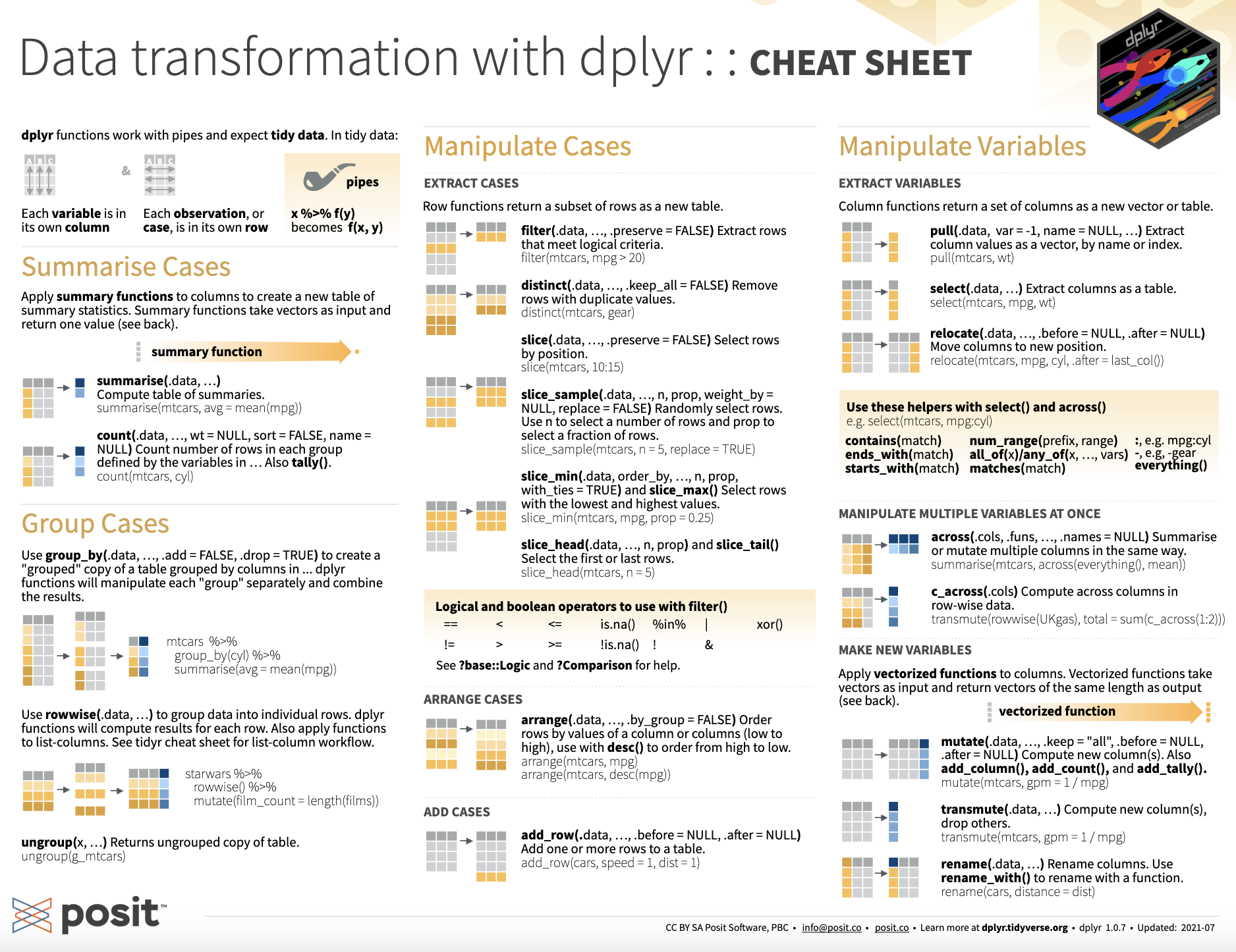
6 Zdbf2 8 6.19The tip of the iceberg
For more, see this handy cheatsheet!
Any questions?
Next, we will learn about data visualization techniques with ggplot2.