library(DESeq2)
library(tidyverse)
library(pheatmap)
Story
The story we’ll work with is a ‘drug repurposing’ effort to use an
old diuretic drug as a cancer treatment:
Amiloride to treat
multiple myeloma
Note that this is publically available data under GEO accession ID
GSE95077, but the data shipped with this repository is altered for
educational purposes.
In this study, RNA-seq data is available to compare amiloride (AMIL) to
a state-of-the-art drug (TG003) in two cancer (multiple myeloma) cell
lines with different mutations (BM: p53mut, JJ: del(17p)).
In total we have 18 samples:
- 3 conditions (drugs): AMIL, TG and DMSO (control)
- 2 cell types: BM and JJ
- 3 replicates for each combination of conditions and cell-types
Design (30 min)
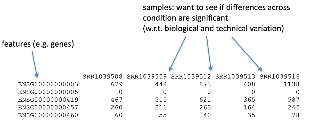
For each gene (=row), the data matrix contains a vector of counts
(\(y\)) which depends on the vector of
samples (\(x\))
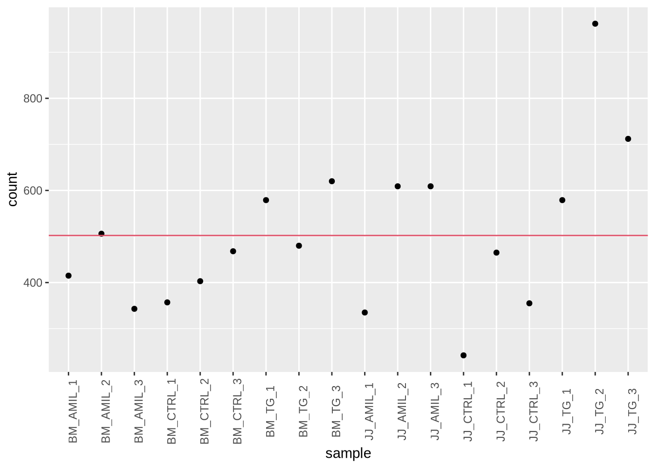
Tasks: Extract the 42nd gene in the data matrix and
plot it against all samples
gene = data %>%
  slice(42) %>%                                                      # pick gene
  pivot_longer(-gene_id, names_to = "sample", values_to = "count")   # convert to long

gene_mean = gene %>% pull(count) %>% mean()                          # calculate mean

ggplot(gene, aes(x=sample, y=count)) +
  geom_point() +
  geom_hline(yintercept = gene_mean, color=2) +
  theme(axis.text.x = element_text(angle = 90))
#base-R
#gene_b = data[42,-1]
#boxplot(gene_b, xlab="sample", ylab="count", names=FALSE)
#abline(h=rowMeans(gene_b), col="red", lty=2)
Hope
Gene expression can be predicted (and controlled) given relevant
sample information \(x\) and a model
\(f(x, \theta)\)
\[
y_i = f(x_i, \theta) ~~~~~~(i = 1\ldots n)\\
\] > Poll 1.5: What is \(n\) in our example?
Qualifications:
- probabilitstic model: predict expectations up to some noise
term \(\to E[y_i] + \epsilon_i\)
- for count data: model the logarithm of the expectation
\(\to \log E[y_i] = f(x_i,
\theta)\)
To keep notation simple we use \(y_i = \log
E[y_i]\) below.
Today we will focus on the function \(f\). Day 2 will cover more about \(\epsilon \propto P(\mu=0, \sigma^2)\)
What should \(x\) be?
Reminder: The researcher needs to decide which
factors should be included in the model.
- none: all samples have their own values \(y\)
- simple average: samples are spread around some global mean \(\to y = \mu + \epsilon\)
- quantitative variable: e.g. sequence depth \(\to y = f(sequencing~depth) +
\epsilon\)
- categorical variable: e.g. condition \(\to
y = f(condition) + \epsilon\)
- combination of variables: e.g. condition and celltype \(\to y = f(condition, celltype) +
\epsilon\)
gene %>%
  # join gene with metadata (by sample)
  inner_join(metadata, by="sample") %>%
  #plot against condition
  ggplot(aes(x=condition, y=count, col=condition)) +
  #geom_point(size=3)  +
  geom_jitter(size = 3, width = 0.1)
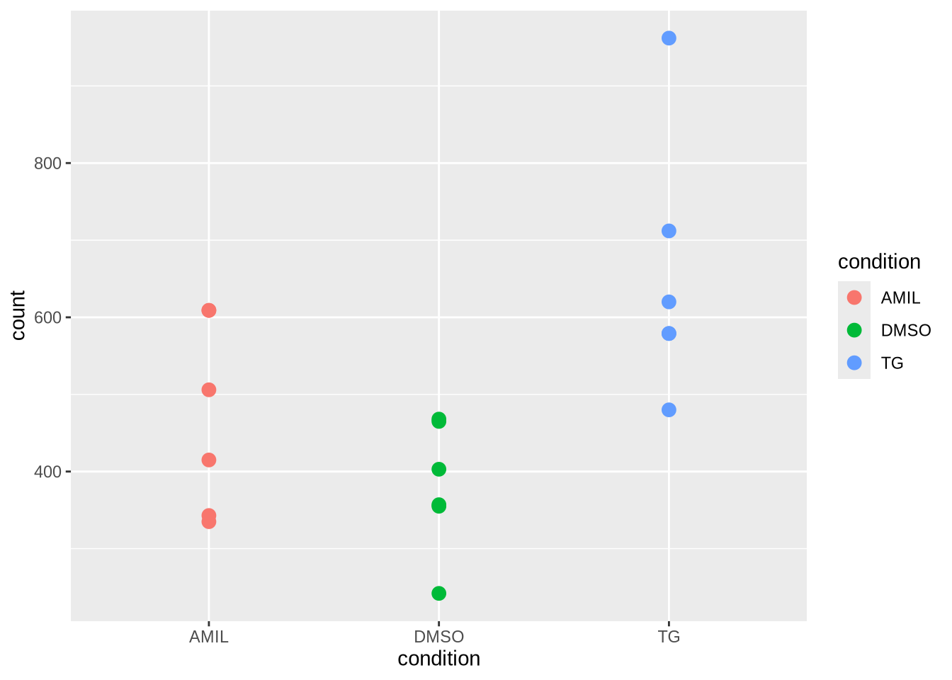
Task: Plot gene counts against celltype.
Notice:
- ggplot understands factors for plotting
- R understands formulae with factors: \(Y
\sim F\)
Under the hood: the model matrix
How are factorial variables (e.g. condition) encoded into something
numerical ?
Use dummy variables: binary encoding of categorical variable \(x\) (switch different levels on and
off)
\[
\left[
\begin{array}{c}
y_1 \\
y_2 \\
\vdots \\
y_i \\
\vdots \\
y_n \\
\end{array}
\right] =
\left[
\begin{array}{ccc}
1 & 0 & \ldots & 0 \\
1 & 0 & \ldots & 0 \\
\vdots \\
0 & 1 & \ldots & 0 \\
\vdots \\
0 & 0 & \ldots & 1 \\
\end{array}
\right] \cdot
\left[
\begin{array}{c}
\mu_1 \\
\mu_2 \\
\vdots \\
\mu_p \\
\end{array}
\right]
\] and in compact notation: \[
y = X \mu
\] \(X\): \(n\times p\) incidence model matrix
\(\to\) multivariate linear
regression.
Recall: \(y=log
E[y]\) so this amounts to a generalized linear regression
(GLM).
An equivalent alternative parameterization is: \[
\left[
\begin{array}{c}
y_1 \\
y_2 \\
\vdots \\
y_i \\
\vdots \\
y_n \\
\end{array}
\right] =
\left[
\begin{array}{ccc}
1 & 0 & \ldots & 0 \\
1 & 0 & \ldots & 0 \\
\vdots \\
1 & 1 & \ldots & 0 \\
\vdots \\
1 & 0 & \ldots & 1 \\
\end{array}
\right] \cdot
\left[
\begin{array}{c}
\beta_0 \\
\beta_1 \\
\vdots \\
\beta_{p-1} \\
\end{array}
\right]
\] and in compact notation: \[
y = \beta_0 + X' \beta
\] \(X'\): \(n \times (p-1)\) model matrix with
intersept. With this parameterization one factor level serves as
reference level \(\beta_0 =
\mu_1\).
Sometimes this choice is preferable since then all the other
parameters \(\beta_i=\mu_{i+1} -
\mu_1\) can be interpreted as effects of level \(i \ge 1\) with respect to reference
level.
We are free to chose from many different parameterizations \(\mu \leftrightarrow \beta\) which will have
different interpretations.
Linear Model
Design In Action
In R, the model matrix \(X\) can be
obtained easily from metadata + design formula. \[
\mbox{R syntax:} ~~~Y \sim V
\]
where the formula should only refer to variables \(V\) that are defined as columns of the
metadata.
metadata %>% colnames
## [1] "sample" "celltype" "condition"
Examples are given below.
Simple designs (1 factor, p-levels)
We may presuppose that gene expression (or rather the logarithm of
the expected counts) is a function of “condition” only
\[
Y \sim condition
\]
Per default this notation refers to equation \(y = \beta_0 + X' \beta\) with an
intercept term \(\beta_0\), but the
latter can also be switched off.
my_design <- ~ 1 + condition   # with intersect (identical to " ~ condition")
my_design <- ~ 0 + condition   # without intersect
The design formula together with a metadata implicitly defines the
model matrix \(X\).
We need \(X\) only occasionally, but
it may be helpful to visualize it here:
X <- model.matrix(my_design, data=metadata)
rownames(X) = metadata$sample
pheatmap(X, cluster_cols = FALSE, cluster_rows=FALSE)
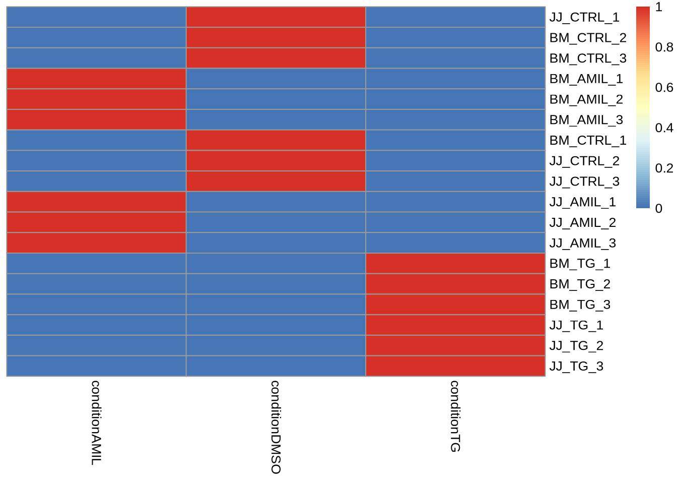
Notice: A factor with \(p\) levels will have \(p\) dummy variables and \(p\) corresponding parameters (e.g. the
means for \(p\) different groups).
Task Try the alternative design formula and inspect
the effect on the matrix.
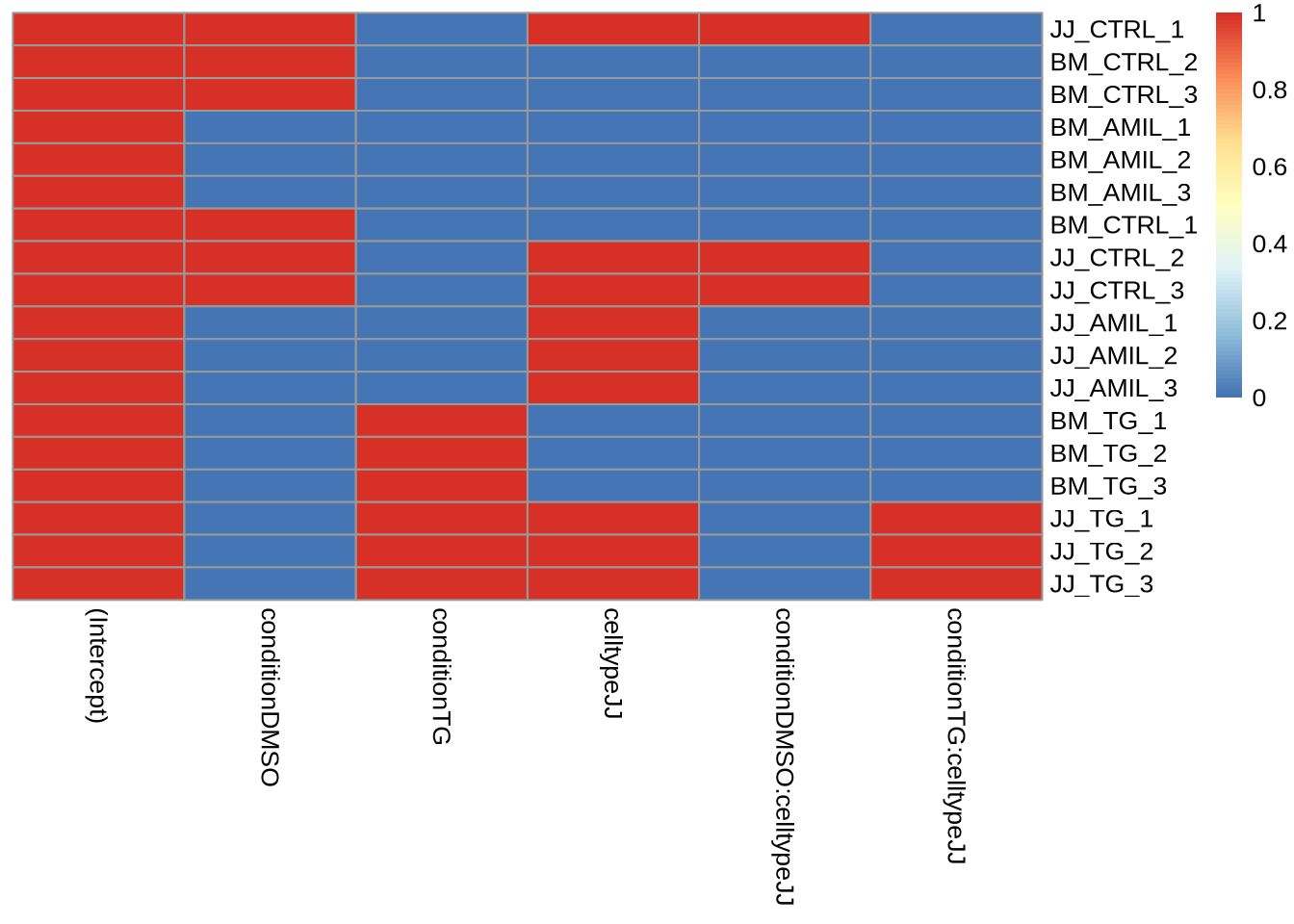
Multifactorial designs
More complicated designs are possible and often necessary (\(\to\) day 2 and 3)
Tasks: Include an additional factor (condition +
celltype) and observe the design matrix
Bonus: Include an interaction term (+
condition*celltype) and discuss its interpretation
X <- model.matrix(~ 1 + condition * celltype, data=metadata)
rownames(X) = metadata$sample
pheatmap(X, cluster_cols = FALSE, cluster_rows=FALSE)
Experimental Design (10 min)
A more elaborate (highly recommended) tutorial can be found here
A typical experiment
The problem: more factors!
Usually there are other factors in addition to a simple
treatment:
- known and interesting: multi-factorial design and interaction
effects (condition * celltype)
- known and uninteresting: batch, covariates
- unknown and unvoidable: noise
… all contribute to total variability and limit our ability to detect
treatment-related differences \(\to\)
account for them as much as possible !
Poll 1.6 You are planning an experiment with 3
treatment levels \((X_1, X_2, X_3)\)
and aim for 3 replicates each. Unfortunately, you can process at most 3
samples per day. So you’ll need three days \((Z_1, Z_2, Z_3)\). How should you assign
your samples to different treatments?
Experimental Design - Poll
Design Checks
For sanity checks it is useful to prepare a table of the metadata
metadata %>% select(-sample) %>% table
##         condition
## celltype AMIL DMSO TG
##       BM    3    3  3
##       JJ    3    3  3
This should answer a few common design questions - even
before any data \(Y\)
is collected !
- Are all cells occupied (full design)?
- Do all cells have the same number of observations (balanced
design)
- Are there missing observations - empty cells?
- Is there confounding between factors?
Sources of Variability
| Source |
What can be done about it ? |
| Treatment |
Control - or observe? |
| Biological |
Estimate with replication |
| Technical |
Control with sequencing depth (read
sampling) |
| Sample Preparation |
Estimate with batch controls
(blocking) |
| Unknown Confounders |
Reduce risk by randomization |
| Errors (e.g. sample swaps) |
Detection, Documentation, SOPs |
| Analysis |
Control software version and
parameters |
Some nuisance factors (e.g. batches) may be known and
measurable, but are not of primary interest - they should be included as
metadata and in the model.
\[
\mbox{R syntax:} ~~~Y \sim X + Z
\]
Reminder: The choice of factors rests with the
researcher.
Factor Choices.
Break (10 min)
Create DESeq2 object (5 min)
Each software has their own data representation :-(
A DESeq2 data object combines data, metadata and the design formula
in one single object
dds = data + metadata + design
All subsequent calculations will use this object (and modify it).
Task: Create a DESeq data set using
DESeq::DESeqDataSetFromMatrix()
dds <- DESeqDataSetFromMatrix(
  # countData= expects matrix, so remove "gene_id" column but keep as rowname
  countData=data %>% column_to_rownames("gene_id"),
  colData=metadata,
  design= my_design)
## converting counts to integer mode
Data Exploration (40 min)
1. Data Access
Tasks:
- Inspect the class, structure and dimensions of
dds.
- Re-extract the count matrix (Hint: ?counts) and save as
Y
- Re-extract the metadata (Hint: ?colData), remove column “sample” and
save as
meta
## class: DESeqDataSet
## dim: 57905 18
## metadata(1): version
## assays(1): counts
## rownames(57905): ENSG00000000003 ENSG00000000005 ... ENSG00000273492
##   ENSG00000273493
## rowData names(0):
## colnames(18): JJ_CTRL_1 BM_CTRL_2 ... JJ_TG_2 JJ_TG_3
## colData names(3): sample celltype condition
Tasks:
- Extract the first 10 rows (genes) from count matrix
Y
and safe this data subset as Yr (reduced size for further
use)
- Optional: Extract 10 randomly sampled genes.
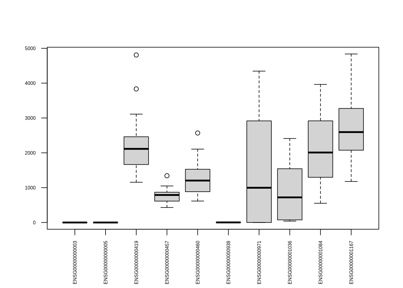
Yr <- Y %>% head(10)                        # extract first 10 rows (for illustrations only)
#Yr <- Y %>% data.frame() %>% sample_n(10)  # random rows
2. Data Visualization
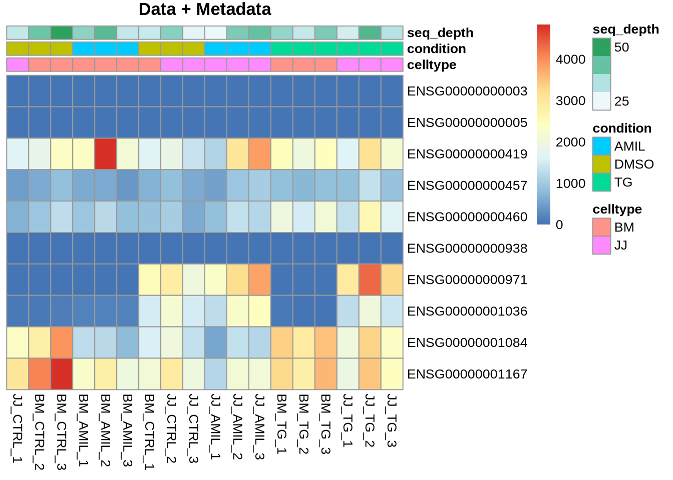
Task: Create heatmap for the reduced data set Yr
(?pheatmap). You might want to disable the default clustering of rows
and columns
pheatmap(Yr, cluster_rows=FALSE, cluster_cols=FALSE, main="First glimpse")
Task: Add metadata meta as annotation
to pheatmap
Customizing Colours (5 min)
Often we need to adjust colours or ensure consistency across a
project. In the example above, the colour representation of the metadata
may also be improved.
Use > library(RColorBrewer) for systematic and educated colour
choices.
Goal: Define list of colours to be used for
metadata?
# celltype colours
ct_col <- c("white", "black")
names(ct_col) <- levels(meta$celltype)
# condition colours
cn_col <- c("#1B9E77", "#D95F02", "#7570B3") # = RColorBrewer::brewer.pal(n=3, "Dark2")
names(cn_col) <- levels(meta$condition)
# create list of colour choices
my_colors <- list( celltype= ct_col, condition = cn_col )
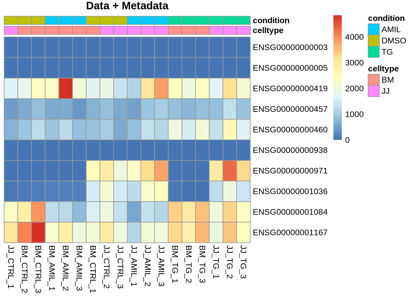
pheatmap(Yr, cluster_rows=FALSE, cluster_cols=FALSE,
annotation=meta, annotation_colors = my_colors,
main="Data + Metadata")
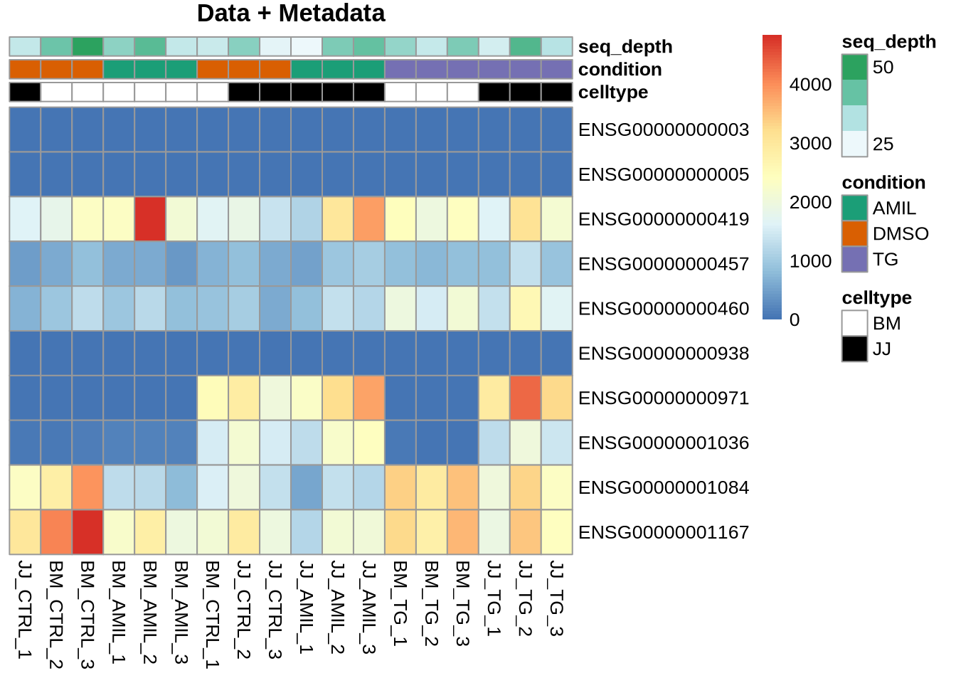
The colour encoding of the heatmap can also be customized (code not
run)
blue_colors = RColorBrewer::brewer.pal(9,"Blues")
pheatmap(Yr, cluster_rows=FALSE, cluster_cols=FALSE,
         annotation = meta, annotation_colors = my_colors,
         color=blue_colors,
         main="Data + Metadata")
4. Sample-Sample correlations
Here the goal is to derive the overall similarity of samples based on
the genome-wide expression data.
Question: How to calculate the sample-sample
correlation matrix?
C <- cor(Yt)       # get sample-sample correlations: other correlations?
pheatmap(C, annotation = meta, annotation_colors = my_colors)
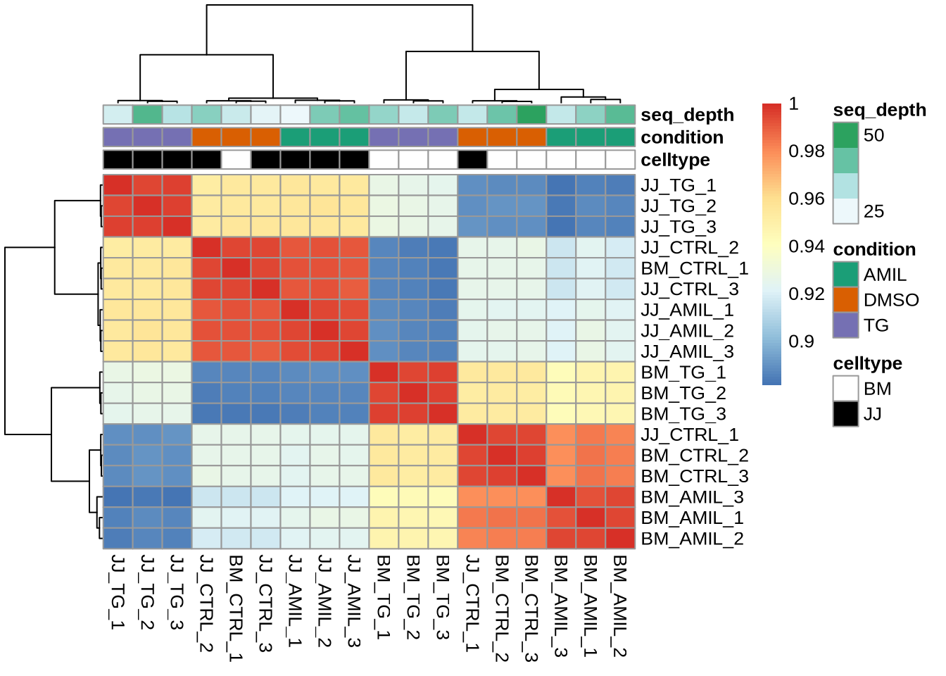
Notice the overall high correlations. How would you explore this
further?
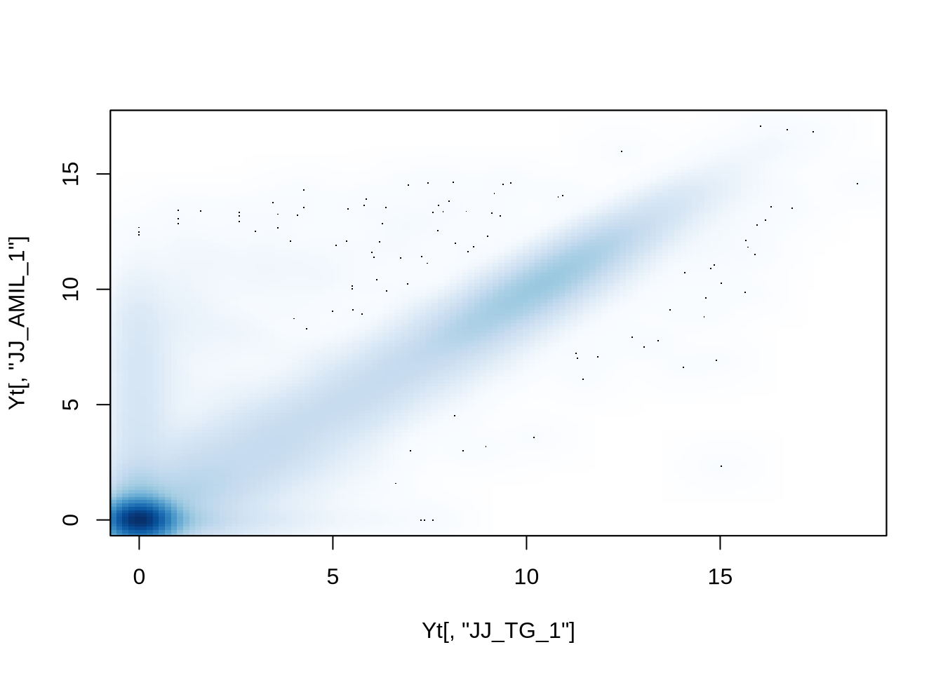
# correlation coeff. is only a single number
smoothScatter(Yt[,"JJ_TG_1"], Yt[,"JJ_AMIL_1"])
5. PCA plot
PCA aims to project samples from a high-dimensional space (M=20k+
genes) to a lower dimension (D=2). Similar to correlation analysis, the
main purpose is to identify distinct and similar samples.
# vst() is one of many variance stabilization methods: log, vst, rlog, ...
# DESeq::plotPCA() requires a 'DESeqTransform' object as input

PCA <- dds %>% vst %>% plotPCA(intgroup=c("condition","celltype"), returnData=TRUE)

# get percentage explained variation per PC
percentVar <- round(100 * attr(PCA, "percentVar"), 1)

ggplot(PCA, aes(x=PC1, y=PC2, color=condition, shape=celltype)) +
  geom_point(size=3, alpha=0.5) +
  xlab(paste0("PC1: ",percentVar[1])) +
  ylab(paste0("PC2: ",percentVar[2]))
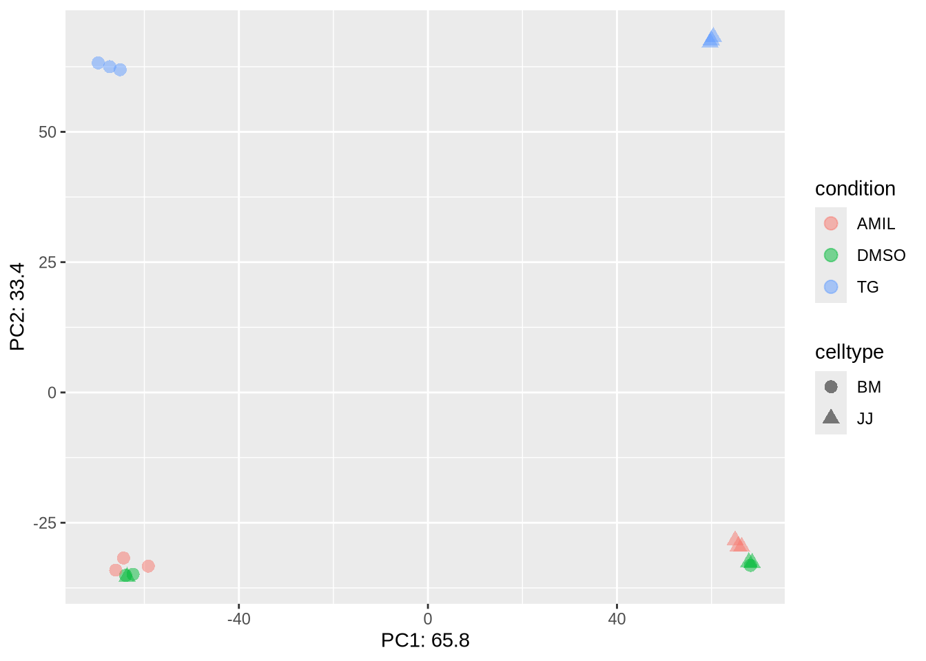
Homework
- Observe and interpret the PCA plot.
- Which factor explains the separation?
- Can we go ahead with analysis ?
- Optional: Repeat PCA analysis with more sophisticated normalization
from the DESeq2 package “rlog()”. Notice that the output is not a matrix
but a more complicated DESeqTransform object.
rld <- rlog(dds)  # more sophisticated log-transform to account for seq.depth=lib.size --> str(rld)

plotPCA(rld)
rld_PCA <- plotPCA(rld, intgroup=c("condition", "celltype"), returnData=TRUE)
percentVar <- round(100 * attr(rld_PCA, "percentVar"), 1)

ggplot(rld_PCA, aes(PC1, PC2, color=condition, shape=celltype)) +
  geom_point(size=3) +
  xlab(paste0("PC1: ",percentVar[1])) +
  ylab(paste0("PC2: ",percentVar[2])) +
  scale_colour_manual(values=cn_col)