DESeq2 Analysis with R: Part 03
Bioinfo-Core @ MPI-IE
Wed Jun 25 06:53:16 2025
Goals: Exploring and defining ‘DESeq2 results’
- repeat: generating DESeq-object (data, metadata, design)
- repeat: run DESeq workflow
- coefficients, contrasts and shrinking
- summarize and visualize results
- LRT vs Wald test
- Biological interpretation
suppressPackageStartupMessages({
library("DESeq2")
library("tidyverse")
library("pheatmap")
library("ggrepel")
library("EnsDb.Hsapiens.v75")
library("UpSetR")
library("ashr")
library("gridExtra")
})
Start by reading countdata, metadata, creating a dds object and performing the filtering as we did yesterday.
data <- readr::read_tsv("data/myeloma/myeloma_counts.tsv")
metadata <- readr::read_tsv("data/myeloma/myeloma_meta.tsv")
metadata <- metadata %>% mutate_if(is.character,as.factor)
dds <- DESeqDataSetFromMatrix(
countData=data %>% column_to_rownames("gene_id"),
colData=metadata,
design=~1
)
dds <- dds[, -c(1,7)]
rs <- dds %>% counts %>% rowSums()
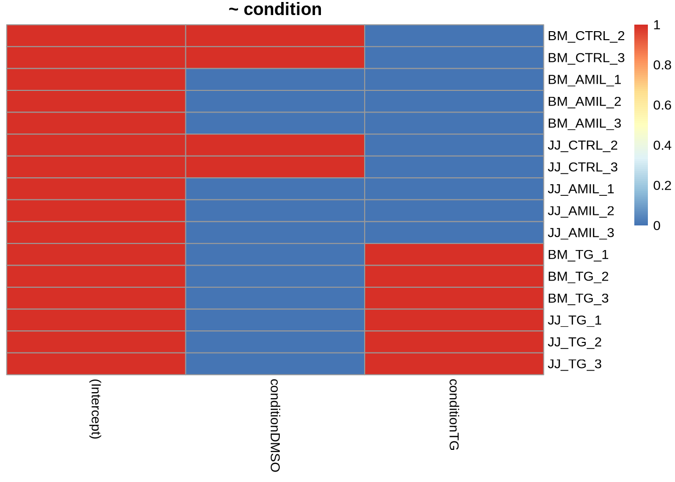
dds <- dds[rs>1,]1. Coefficients and design (30 minutes)
a. factors and design
Remember that ideally all sources of variation to control should be specified in the design. Also recall that we saw two different ways to specify (‘parametrize’) our model.
~ condition == ~ 1 + condition
\[ y_{ij} = \beta_0 + \beta_1X_1 + ... + \beta_kX_k + \epsilon_{ij} \] where K = i - 1
pheatmap(
  model.matrix(~condition, data=colData(dds)),
  cluster_cols = FALSE,
  cluster_rows=FALSE,
  main="~ condition"
)
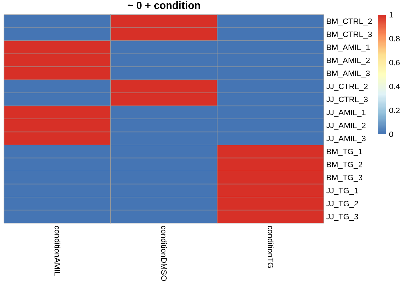
~ 0 + condition
\[ y_{ij} = \mu_i + \epsilon_{ij} \]
pheatmap(
  model.matrix(~ 0 + condition, data=colData(dds)),
  cluster_cols = FALSE,
  cluster_rows=FALSE,
  main="~ 0 + condition"
)
b. design examples
A single factor with two levels - intercept
| samples | celltype |
|---|---|
| sample1 | JJ |
| sample2 | JJ |
| sample3 | BM |
| sample4 | BM |
design(dds) <- ~celltype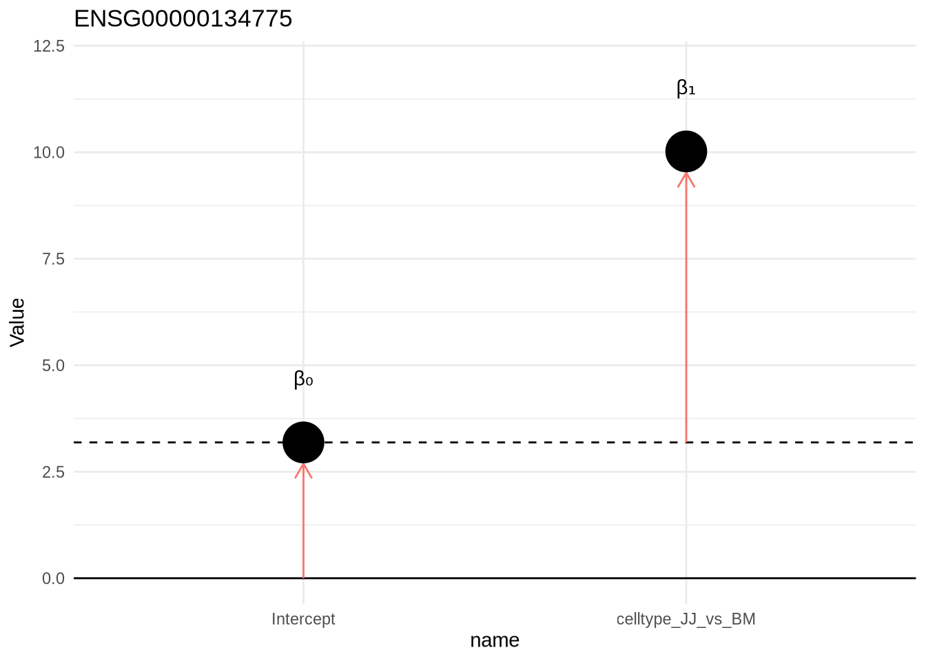
dds <- DESeq(dds)resultsNames(dds)## [1] "Intercept" "celltype_JJ_vs_BM"Design:
  ~1 + celltype (or ~celltype)
  expression = beta0 + beta1 * JJ
Our coefficients here are our intercept, and condition for our celltype effect versus the base level. Remember, the base level is the first level in your celltype factor (which by default is alphabetically determined).
Poll 3.1 What does the intercept (beta0) value reflect ?
dds$celltype## [1] BM BM BM BM BM JJ JJ JJ JJ JJ BM BM BM JJ JJ JJ
## Levels: BM JJEach coefficient shows a difference.
[1] "Intercept" (beta0) "celltype_JJ_vs_BM" (beta1)This can be shown by dummy variables:
| samples | (Intercept) | celltypeJJ |
|---|---|---|
| sample1 | 1 | 0 |
| sample2 | 1 | 0 |
| sample3 | 1 | 1 |
| sample4 | 1 | 1 |
Null hypothesis:
BM vs JJ
beta1 = 0
A single factor with two levels - no intercept
Let’s look at the same setup, but this time omit our intercept
design(dds) <- ~0+celltype
dds <- DESeq(dds)resultsNames(dds)## [1] "celltypeBM" "celltypeJJ"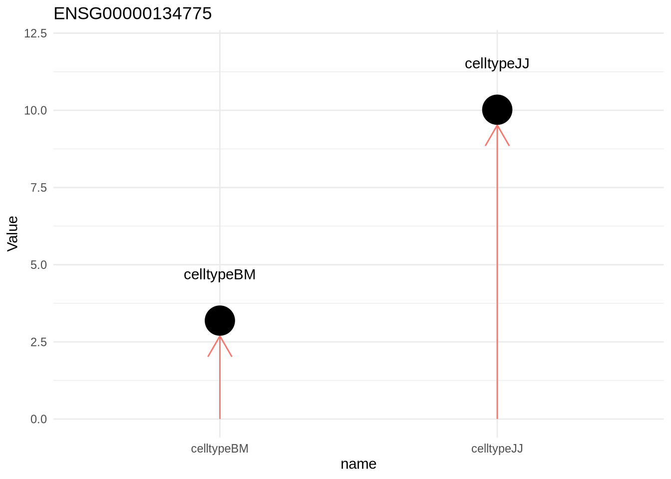
A single factor with more than two levels - intercept
| samples | condition |
|---|---|
| sample1 | AMIL |
| sample2 | AMIL |
| sample3 | DMSO |
| sample4 | DMSO |
| sample5 | TG |
| sample6 | TG |
Tasks: Recreate the dds object, now with a design that incorporates ‘condition’ AND an intercept.
Poll 3.2 What coefficients do we get when we specify ‘condition’ alone as a design?
design(dds) <- ~condition
dds <- DESeq(dds)resultsNames(dds)## [1] "Intercept" "condition_DMSO_vs_AMIL" "condition_TG_vs_AMIL"Design:
  ~1+condition
  = beta0 + beta1 * DMSO + beta2 * TG
  beta0 = Intercept
  beta1 = condition_DMSO_vs_AMIL
beta2 = condition_TG_vs_AMIL 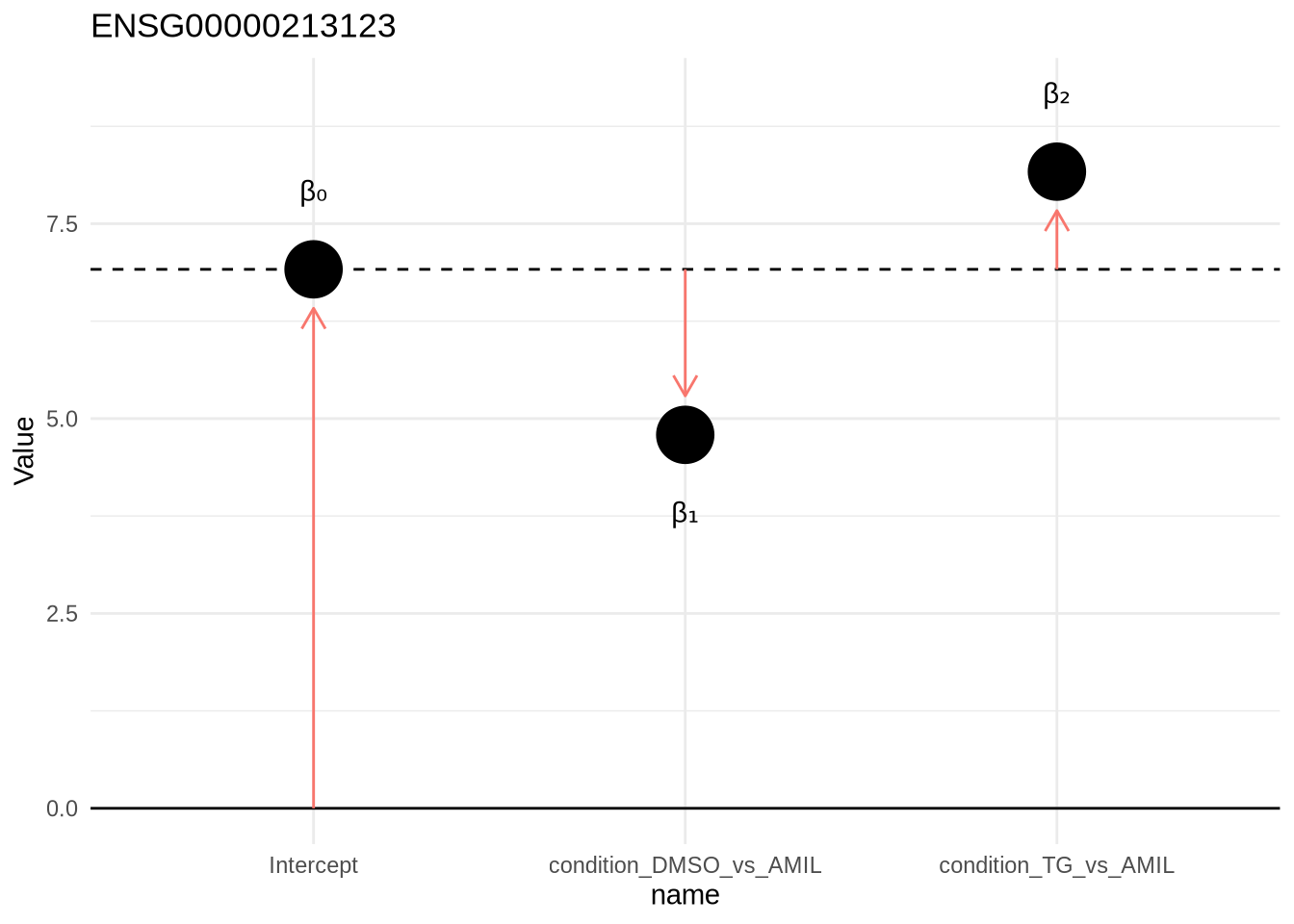
Model matrix:
| samples | (Intercept) | conditionDMSO | conditionTG |
|---|---|---|---|
| sample1 | 1 | 0 | 0 |
| sample2 | 1 | 0 | 0 |
| sample3 | 1 | 1 | 0 |
| sample4 | 1 | 1 | 0 |
| sample5 | 1 | 0 | 1 |
| sample6 | 1 | 0 | 1 |
Null hypothesis:
AMIL vs DMSO
beta1 = 0

AMIL vs TG
beta2 = 0

DMSO vs TG
beta1 - beta2 = 0
A single factor with more than two levels - no intercept
Let’s again look at the scenario where we don’t include an intercept.
design(dds) <- ~0+condition
dds <- DESeq(dds)resultsNames(dds)## [1] "conditionAMIL" "conditionDMSO" "conditionTG"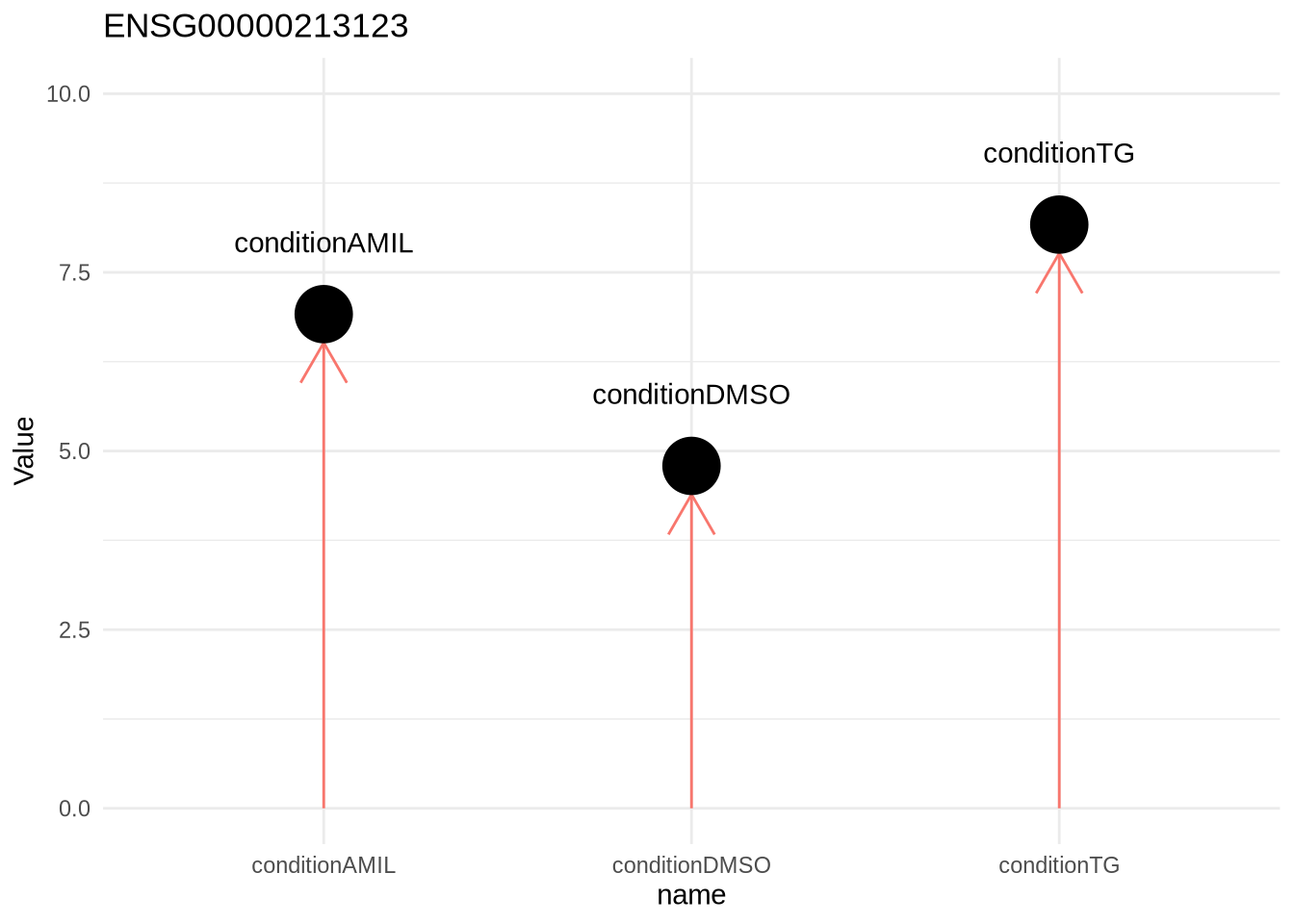
two factors, with an interaction - intercept
What about celltype and condition?
- Two factors, with interaction
| samples | celltype |
condition |
|---|---|---|
| sample1 | JJ | AMIL |
| sample2 | JJ | AMIL |
| sample3 | JJ | DMSO |
| sample4 | JJ | DMSO |
| sample5 | JJ | TG |
| sample6 | JJ | TG |
| sample7 | BM | AMIL |
| sample8 | BM | AMIL |
| sample9 | BM | DMSO |
| sample10 | BM | DMSO |
| sample11 | BM | TG |
| sample12 | BM | TG |
The formula for the model includes all sources of variation in the data. Thus, it should contain the celltype, condition and the difference as the effect of celltype on the condition (celltype:condtion)
Design:
~1 + celltype + condition + celltype:condition
= beta0 + beta1 * JJ + beta2 * DMSO + beta3 * TG + beta4 * JJ.DMSO + beta4 * JJ.TG

  beta0 = Intercept
  beta1 = celltype_JJ_vs_BM
  beta2 = condition_DMSO_vs_AMIL
  beta3 = condition_TG_vs_AMIL
  beta4 = celltypeJJ.conditionDMSO
  beta5 = celltypeJJ.conditionTG
design(dds) <- ~celltype+condition+celltype:condition
dds <- DESeq(dds)resultsNames(dds)## [1] "Intercept" "celltype_JJ_vs_BM"
## [3] "condition_DMSO_vs_AMIL" "condition_TG_vs_AMIL"
## [5] "celltypeJJ.conditionDMSO" "celltypeJJ.conditionTG"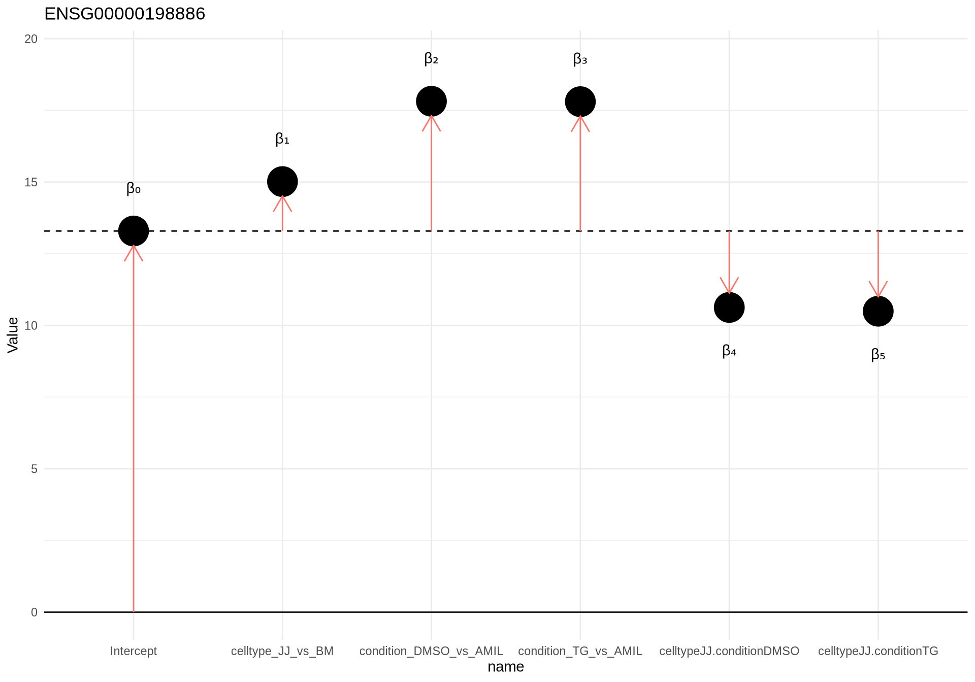
Poll 3.3 What does the intercept value reflect ?
Null hypothesis:
BM vs JJ (AMIL!)
beta1 = 0

BM vs JJ (DMSO!)
beta1 + beta4 = 0

AMIL vs DMSO (BM):
beta2 = 0

DMSO vs TG (BM):
beta2 + beta3 = 0Reminder: The levels of your factors define which ‘baseline’ will be used, and thus what coefficients you will have!
- Multi-factor design with increasing complexity are nicely explained in Hugo Tavares’ slides
two factors, with an interaction - no intercept
design(dds) <- ~0+celltype:condition
dds <- DESeq(dds)resultsNames(dds)## [1] "celltypeBM.conditionAMIL" "celltypeJJ.conditionAMIL"
## [3] "celltypeBM.conditionDMSO" "celltypeJJ.conditionDMSO"
## [5] "celltypeBM.conditionTG" "celltypeJJ.conditionTG"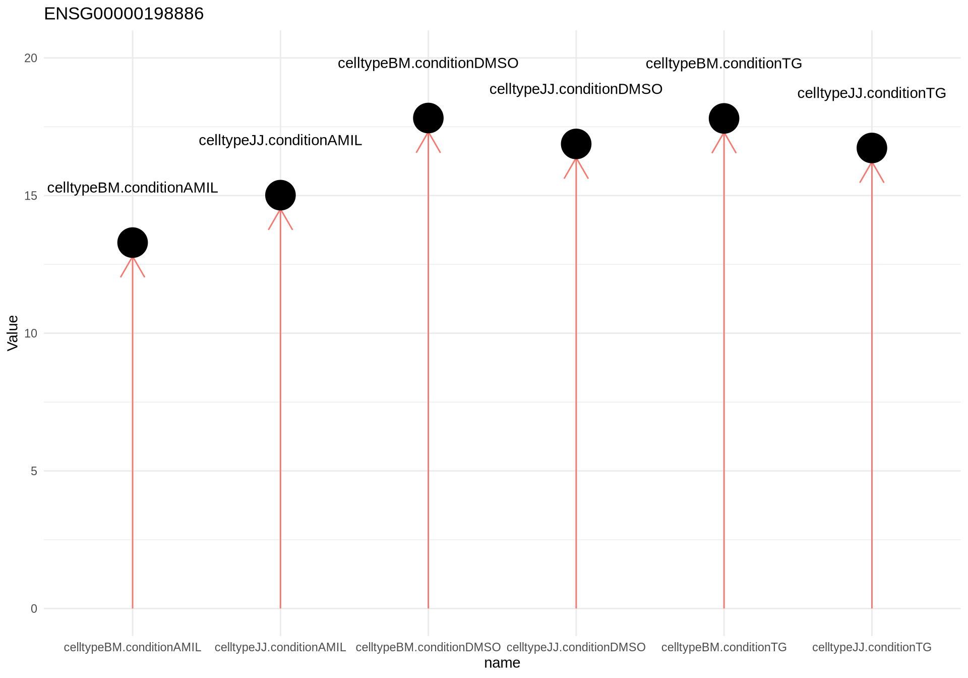
Note that the variables of interest in your design can also be ‘nuisance’ factors, for example batch effects. It’s important to include those in the design (cfr. day 01). To subsequently get the comparisons of interest, one can refer to proper contrasts or coefficients of interest (see below). If one imagines that our celltype variable is a ‘batch effect’ (i.e. samples prepared on Monday, or on Saturday), it’s clear that not including batch in the design would lead to an increased variance estimation.
c. Recap
Build object
data <- readr::read_tsv("data/myeloma/myeloma_counts.tsv")
metadata <- readr::read_tsv("data/myeloma/myeloma_meta.tsv")
metadata <- metadata %>% mutate_if(is.character,as.factor)

dds <- DESeqDataSetFromMatrix(
  countData=data %>% column_to_rownames("gene_id"),
  colData=metadata,
  design=~celltype+condition+celltype:condition
)
dds <- dds[, -c(1,7)]
rs <- dds %>% counts %>% rowSums()
dds <- dds[rs>1,]
dds <- estimateSizeFactors(dds)
sizeFactors(dds)## BM_CTRL_2 BM_CTRL_3 BM_AMIL_1 BM_AMIL_2 BM_AMIL_3 JJ_CTRL_2 JJ_CTRL_3 JJ_AMIL_1
## 1.1433547 1.4178968 1.1081712 1.2521730 0.8317523 1.0132260 0.6720967 0.6667752
## JJ_AMIL_2 JJ_AMIL_3 BM_TG_1 BM_TG_2 BM_TG_3 JJ_TG_1 JJ_TG_2 JJ_TG_3
## 1.0994127 1.2136785 1.1125837 0.9072609 1.1596233 0.7719960 1.2800491 0.9103010Reminder: Note that you can intervene at this stage to override the size factor calculation (for example with spike in calculated size factors).
dds <- estimateDispersions(dds)
plotDispEsts(dds)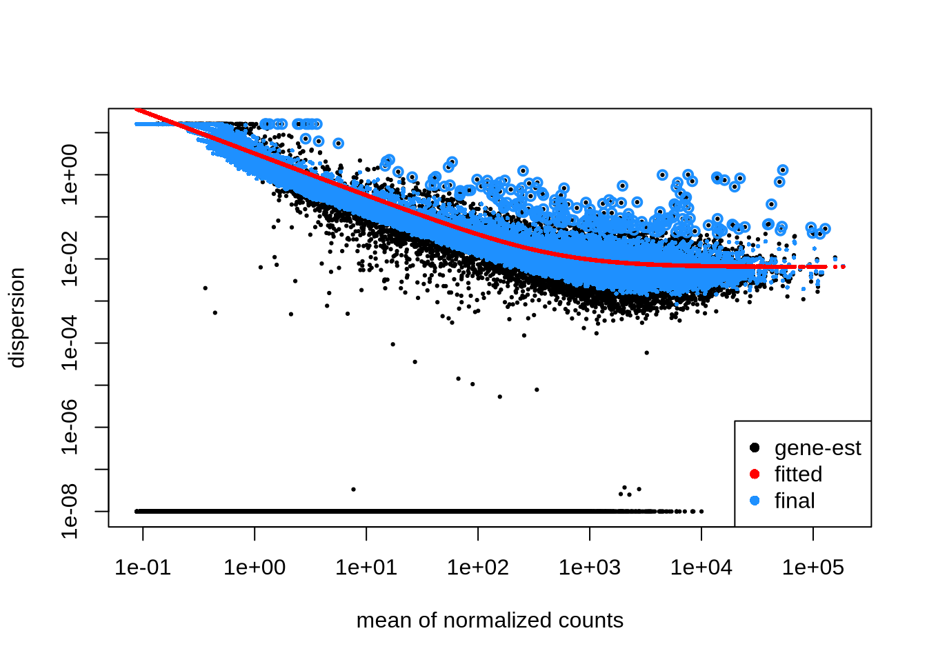
dds <- nbinomWaldTest(dds)Or everything in 1 go
dds <- DESeq(dds)2. Give me results! (30 min)
a. Wald test
By default DESeq2 uses the Wald test to identify genes that are differentially expressed between two groups of samples. This is done through the following steps:
- A regression model fits to each gene (glm.nb),
- Each gene model coefficient (LFC) is estimated using a maximum likelihood estimation,
- The shrunken estimate of LFC is divided by its standard error, resulting in a z-statistic,
- z-statistic is compared to a standard normal distribution to compute the p-values,
- P values are adjusted for multiple testing
res_dds <- results(dds) %>% data.frame()
res_dds[c("ENSG00000001626", "ENSG00000130985", "ENSG00000100596", "ENSG00000196700", "ENSG00000039987"),] %>% arrange(log2FoldChange)
A frequently asked question is: ‘Why is my padj ’NA’ but my p-values are significant ? It’s my favorite gene!’
There are three reasons to set adjusted p-values to NA (From the DESeq2 vignette)
- within a row, all samples have zero counts (remember that we filtered these, so this doesn’t apply here !)
- a row contains a sample with an extreme count outlier
- A row is filtered by independent filtering (in essence a count cut-off).
p1 <- ggplot() +
  geom_point(size=0.5, aes(x=log10(res_dds$baseMean), y=-log10(res_dds$padj))) +
  theme_minimal() +
  ggtitle("Independent filtering") +
  xlab("log10(baseMean)") +
  ylab("-log10(padj)")
p2 <- ggplot() +
  geom_point(size=0.5, aes(x=log10(res_dds$baseMean), y=-log10(p.adjust(res_dds$pvalue, method='hochberg')))) +
  theme_minimal() +
  ggtitle("No independent filtering") +
  ylab("-log10(padj)") +
  xlab("log10(baseMean)")
grid.arrange(p1, p2, nrow=1)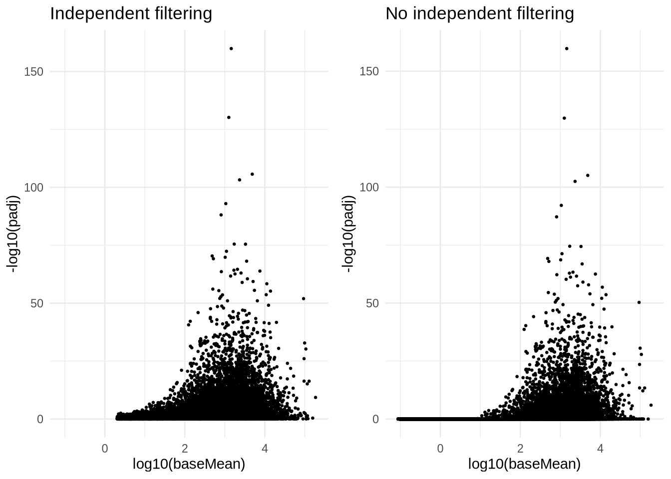
We have called results here, but what did we actually compare ?
resultsNames(dds)## [1] "Intercept" "celltype_JJ_vs_BM"
## [3] "condition_DMSO_vs_AMIL" "condition_TG_vs_AMIL"
## [5] "celltypeJJ.conditionDMSO" "celltypeJJ.conditionTG"Reminder:
If ‘results’ is run without specifying ‘contrast’ or ‘name’, the last coefficient will be tested. In this case ‘celltypeJJ.conditionDMSO’.
b. Contrasts and results
Contrasts are used in our results call to get a specific comparison. If there is only one factor with two levels, There is no need to specify contrasts, DESeq2 will choose the base factor level based on the alphabetical order of the levels.
Contrasts can be specified in three different ways:
- a character vector with three elements. c(“celltype”, “JJ”, “BM”) (last level == baseline!)
- A list of 2 characters, corresponding to the coefficients. list(coef1, coef2)
- A numerical vector with an element for each coefficient. c(0,0,0,1,0,0)
Let’s try!
Specify a c("condition", "AMIL", "DMSO") contrast in the
result function:
contrast <- c("condition", "DMSO", "AMIL")
res <- results(dds, contrast = contrast)
res <- res %>% data.frame() %>% drop_na()
res %>% head()
Columns of results dataframe:
baseMean: mean of normalized counts for all samples
log2FoldChange: log2 fold change
lfcSE: standard error
stat: Wald statistic
pvalue: Wald test p-value
padj: BH adjusted + independently filtered p-values
Note that we are testing the the Amiloride effect (with DMSO as a baseline) under the base-levels of all other factors in the model. In this case this corresponds to a DMSO - Amiloride comparison in BM cells.
sig_genes <- res %>% arrange(padj) %>% dplyr::filter(padj < 0.05)
nonsig_jj <- c(
"ENSG00000002016","ENSG00000002549", "ENSG00000004139", "ENSG00000004838",
"ENSG00000005007", "ENSG00000005022", "ENSG00000005102", "ENSG00000005469",
"ENSG00000005884", "ENSG00000005889", "ENSG00000006114", "ENSG00000006194",
"ENSG00000006459", "ENSG00000006652", "ENSG00000007047"
)
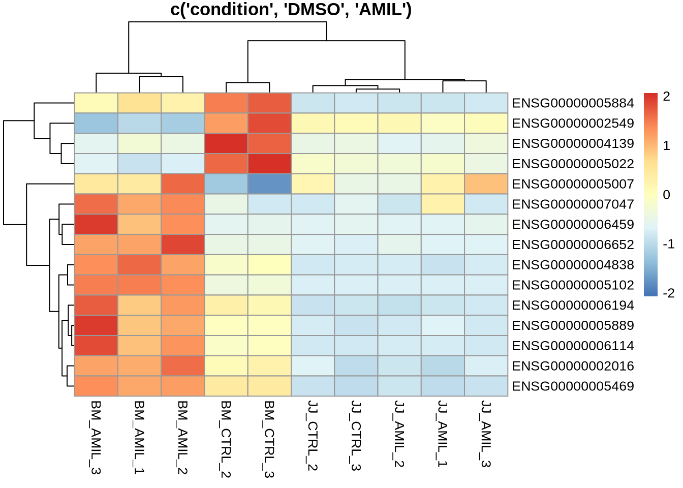
pheatmap(counts(dds, normalized=T)[
sig_genes[nonsig_jj,] %>% rownames(),
c("BM_CTRL_2", "BM_CTRL_3", "BM_AMIL_1", "BM_AMIL_2", "BM_AMIL_3",
"JJ_CTRL_2", "JJ_CTRL_3", "JJ_AMIL_1", "JJ_AMIL_2", "JJ_AMIL_3")
],
scale='row',
main='c(\'condition\', \'DMSO\', \'AMIL\')'
)
Let’s look at a ‘list’ example. by asking ‘condition_DMSO_vs_AMIL’ we ask for the DMSO effect (relative to AMIL), and ‘celltypeJJ.conditionDMSO’ we ask for the DMSO effect in JJ cells.
res2 <- results(dds, contrast = list(c("condition_DMSO_vs_AMIL", "celltypeJJ.conditionDMSO")), alpha = 0.05)
res2 <- res2 %>% data.frame %>% drop_na()
res2 %>% head()
sig_genes <- res2 %>% arrange(padj) %>% dplyr::filter(padj < 0.05)
nonsig_bm <- c(
"ENSG00000003147", "ENSG00000003989", "ENSG00000004142", "ENSG00000005189",
"ENSG00000006468", "ENSG00000006576", "ENSG00000007080",
"ENSG00000008256", "ENSG00000008311", "ENSG00000008323", "ENSG00000008405", "ENSG00000008513", "ENSG00000008517",
"ENSG00000012779", "ENSG00000013275", "ENSG00000013810", "ENSG00000014257"
)
pheatmap(counts(dds, normalized=T)[
sig_genes[nonsig_bm,] %>% rownames(),
c("BM_CTRL_2", "BM_CTRL_3", "BM_AMIL_1", "BM_AMIL_2", "BM_AMIL_3",
"JJ_CTRL_2", "JJ_CTRL_3", "JJ_AMIL_1", "JJ_AMIL_2", "JJ_AMIL_3")
],
scale='row',
cluster_cols=F,
main='list(c(\"condition_DMSO_vs_AMIL\", \"celltypeJJ.conditionDMSO\"))'
)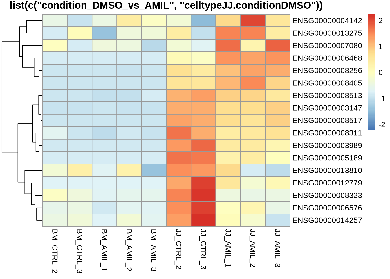 ***
***
And finally, let’s have a look at a numerical contrast.
print(resultsNames(dds))## [1] "Intercept" "celltype_JJ_vs_BM"
## [3] "condition_DMSO_vs_AMIL" "condition_TG_vs_AMIL"
## [5] "celltypeJJ.conditionDMSO" "celltypeJJ.conditionTG"res3 <- results(dds, contrast = c(0,0,1,0,1,0), alpha = 0.05)
res3 <- res3 %>% data.frame %>% drop_na()ggplot() +
geom_point(aes(x=res2$log2FoldChange, y=res3$log2FoldChange)) +
theme_minimal() +
ylab("c(0,0,1,0,1,0)") +
xlab("list(c(\"condition_DMSO_vs_AMIL\", \"celltypeJJ.conditionDMSO\"))")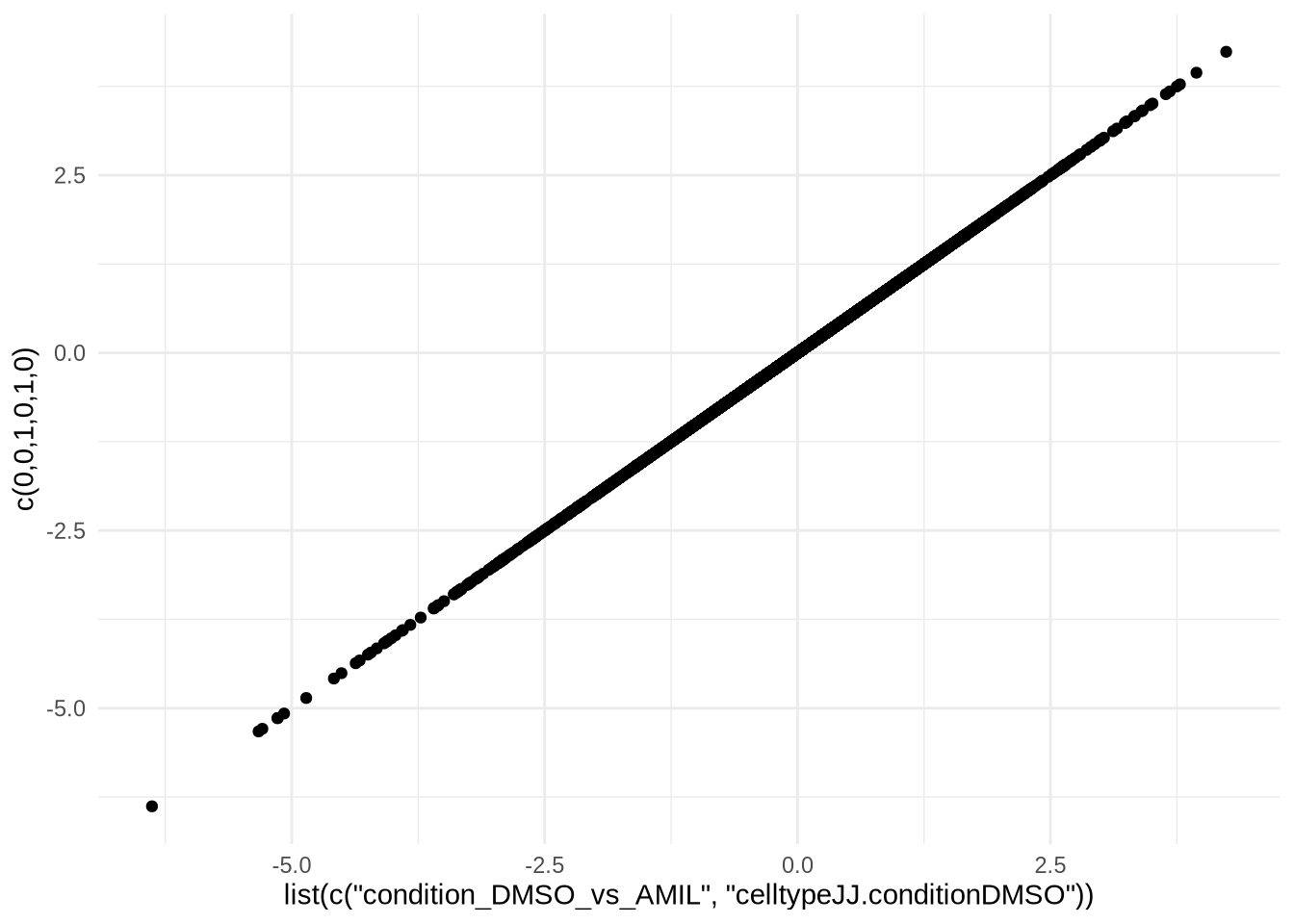
Let’s make some exploratory plots.
ggplot(data=res) +
  geom_point(
    size=0.5,
    color = ifelse(res$padj < 0.05, '#f62728', '#7f7f7f'),
    aes(x=log2FoldChange, y=-log10(padj))
  ) +
  theme_minimal()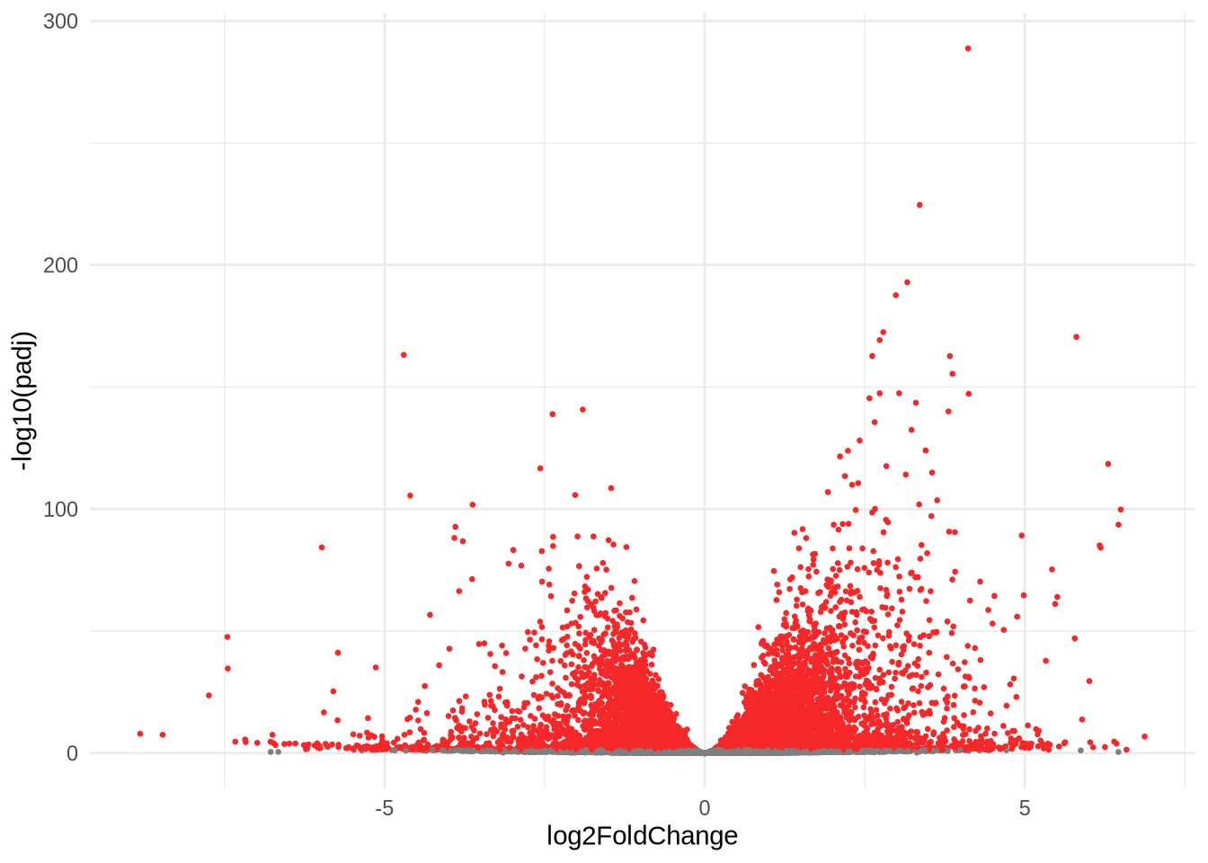
ggplot(data=res) +
  geom_point(
    size=0.5,
    color = ifelse(res$padj < 0.05, '#f62728', '#7f7f7f'),
    aes(x=log10(baseMean), y=log2FoldChange)
  ) +
  theme_minimal()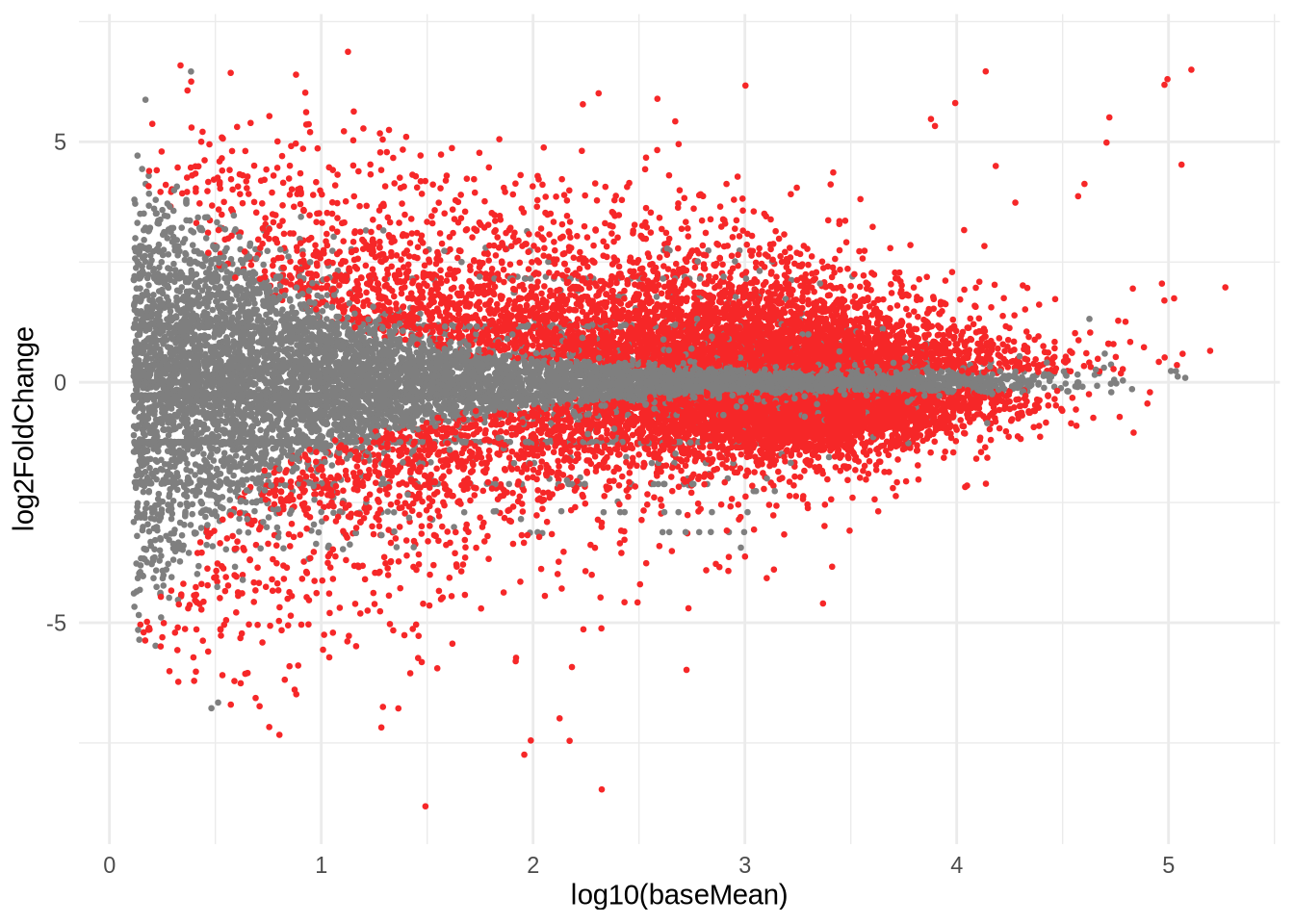
c. Shrinking
To generate more accurate log2 foldchange (LFC) estimates, DESeq2 allows for the shrinkage of the LFC estimates toward zero when the information for a gene is low, which could include:
- Low counts
- High dispersion values
LFC shrinkage generates a more accurate estimate. It looks at the largest fold changes that are not due to low counts and uses these to inform a prior distribution. The genes with little information or high dispersion are then more likely to be assigned to a lower shrunk LFC.
print(contrast)## [1] "condition" "DMSO" "AMIL"res <- results(dds, contrast=contrast)
res_shrink <- lfcShrink(dds, contrast=contrast, type="ashr")Note that there are three ‘built-in’ methods for shrinking:
- normal -> works only with design that have no interaction
- apeglm -> works only with coefficients ! (might have to relevel)
- ashr
The specifics about these methods is beyond the scope of this course.
Recommendation: ashr works for most (if not all) setups, including contrasts.
p1 <- ggplot(data=res %>% data.frame(), aes(x=log10(baseMean + 1), y=log2FoldChange)) +
  geom_point(size=0.5, color=ifelse(data.frame(res)$padj < 0.05, '#f62728', '#7f7f7f')) +
  theme_minimal() +
  ggtitle("un-shrunk")

p2 <- ggplot(data=res_shrink %>% data.frame(), aes(x=log10(baseMean + 1), y=log2FoldChange)) +
  geom_point(size=0.5, color=ifelse(data.frame(res_shrink)$padj < 0.05, '#f62728', '#7f7f7f')) +
  theme_minimal() +
  ggtitle("shrunk")

grid.arrange(p1, p2, nrow=1)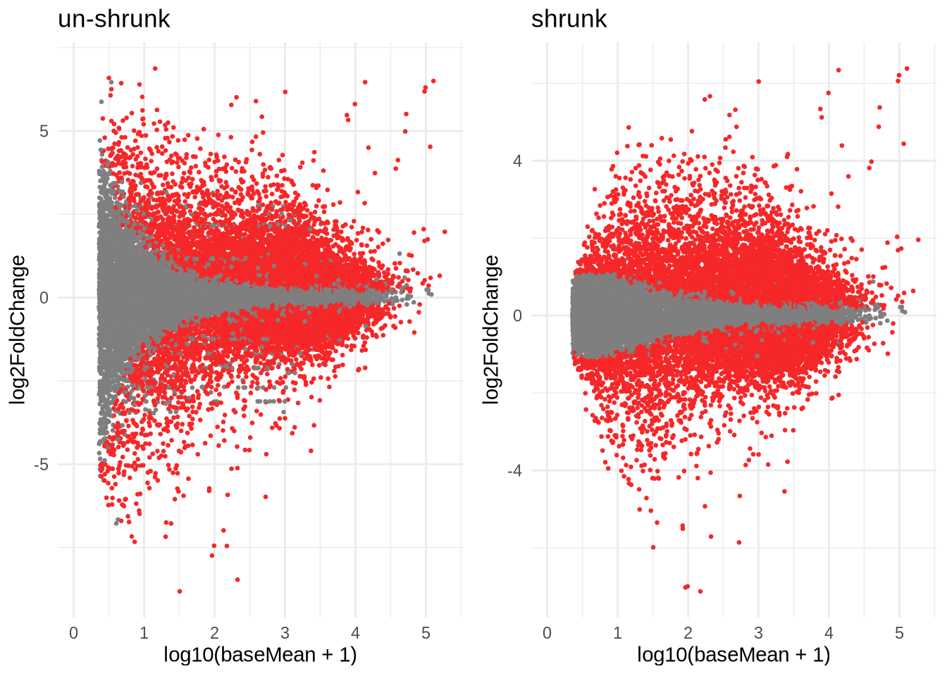
Note: Please run the lfcShrink, so you have the res_shrink object in memory for later !
Break (10 min)
3. Biological interpretation (60 min)
a. Visualisation
You can plot the (normalized) counts of a single gene over your conditions.
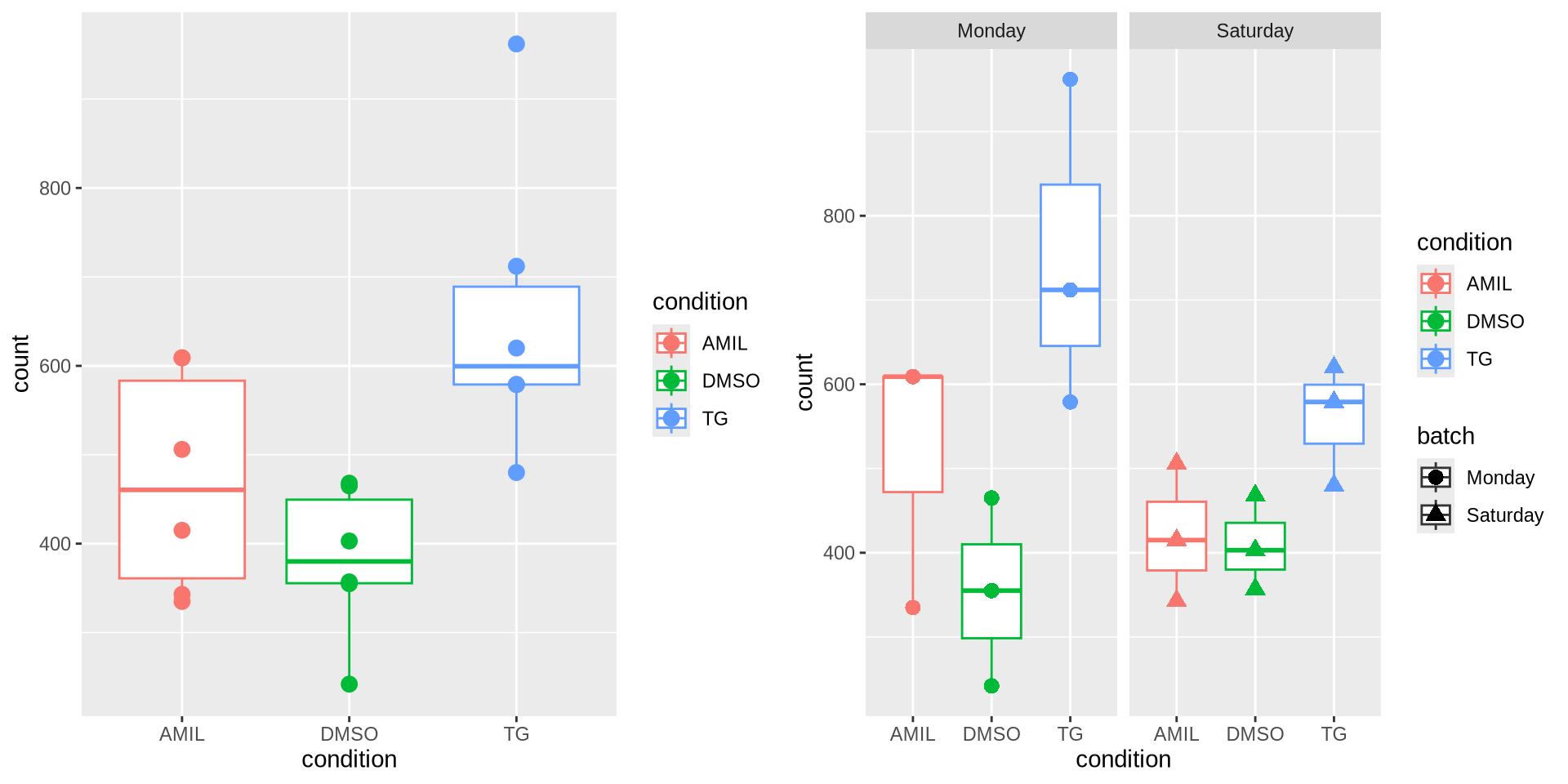
d <- plotCounts(dds, gene = "ENSG00000164062", intgroup = "celltype", returnData=TRUE)
d %>% head()
# can be used for ggplot
ggplot(d, aes(x = celltype, y = count, color = celltype)) +
geom_point(position=position_jitter(w = 0.1,h = 0)) +
geom_text_repel(aes(label = rownames(d))) +
theme_minimal() +
ggtitle("ENSG00000164062") +
theme(plot.title = element_text(hjust = 0.5))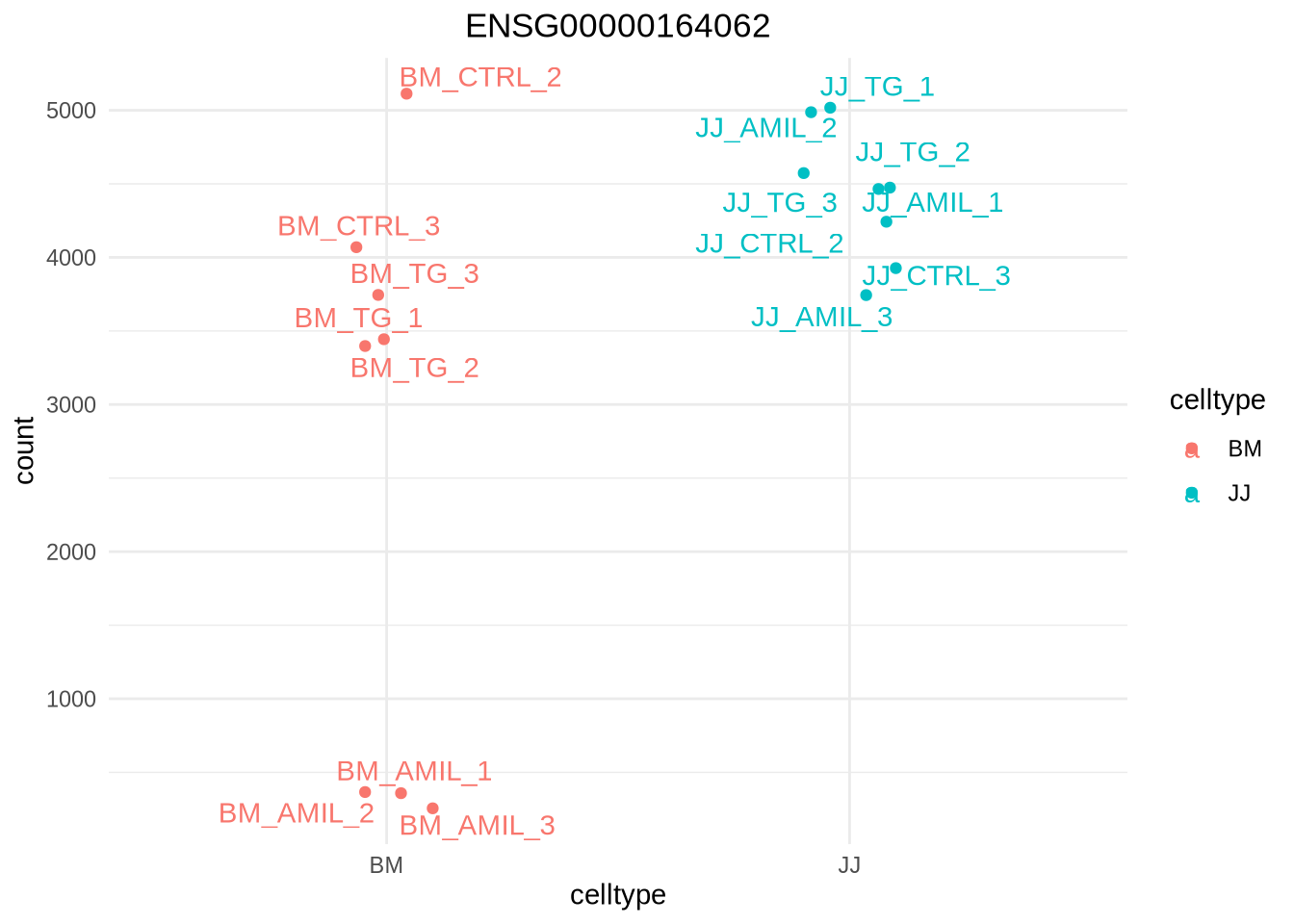
We saw how to create heatmap multiple times, let’s make another !
Task: Plot a heatmap of the normalized counts for the ‘top 20’ genes from our previously generated res_shrink object. (15 minutes)
- convert the res_shrink object to a dataframe ( data.frame() ), sort
by padj( arrange() ), take the top 20 ( head() )
- Extract the normalized (!) counts from the dds object and convert to
dataframe ( counts(dds) )
- subset the dataframe with normalized counts for the gene ID’s in the
top20 ( filter() )
- plot with pheatmap, note that you can scale the values per row (scale=‘row’)!
Reminder: Some function between ensembldb (part of EnsDb.Hsapiens.v79) and dplyr overlap. Explicitly state the library when calling them to avoid errors.
top20 <- res_shrink %>% data.frame() %>% subset(padj < 0.05) %>% arrange(padj, descending=FALSE) %>% head(20)
top20 %>% head()
normcounts <- dds %>% counts(normalized=TRUE) %>% data.frame()
normcounts %>% head()top20_counts <- normcounts %>% dplyr::filter(rownames(normcounts) %in% rownames(top20))
top20_counts %>% head()pheatmap(top20_counts,
cluster_rows = T,
show_rownames = F,
border_color = NA,
fontsize = 10,
scale = "row",
fontsize_row = 10,
height = 20)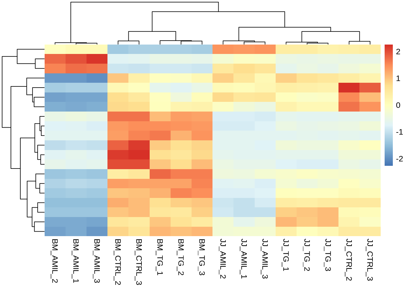
Before the break we also saw an example of an MAplot and a volcano plot. Both are commonly used plots to have a global view of the expression changes.
- volcano plot; in which the log transformed adjusted p-values plotted
on the y-axis and log2 fold change values on the x-axis.
- MAplot; in which the log2FoldChanges are plotted on the y-axis, and the mean expression (log-transformed) on the x-axis.
p1 <- ggplot(data=res_shrink %>% data.frame(), aes(x=log2FoldChange, -log10(padj))) +
  geom_point(size=0.5, color=ifelse(data.frame(res_shrink)$padj < 0.05, '#d62728', '#7f7f7f')) +
  #ylim(c(0,10)) +
  theme_minimal()

p2 <- ggplot(data=res_shrink %>% data.frame(), aes(y=log2FoldChange, x=log10(baseMean))) +
  geom_point(size=0.5, color=ifelse(data.frame(res_shrink)$padj < 0.05, '#d62728', '#7f7f7f')) +
  theme_minimal()

grid.arrange(p1, p2, nrow=1)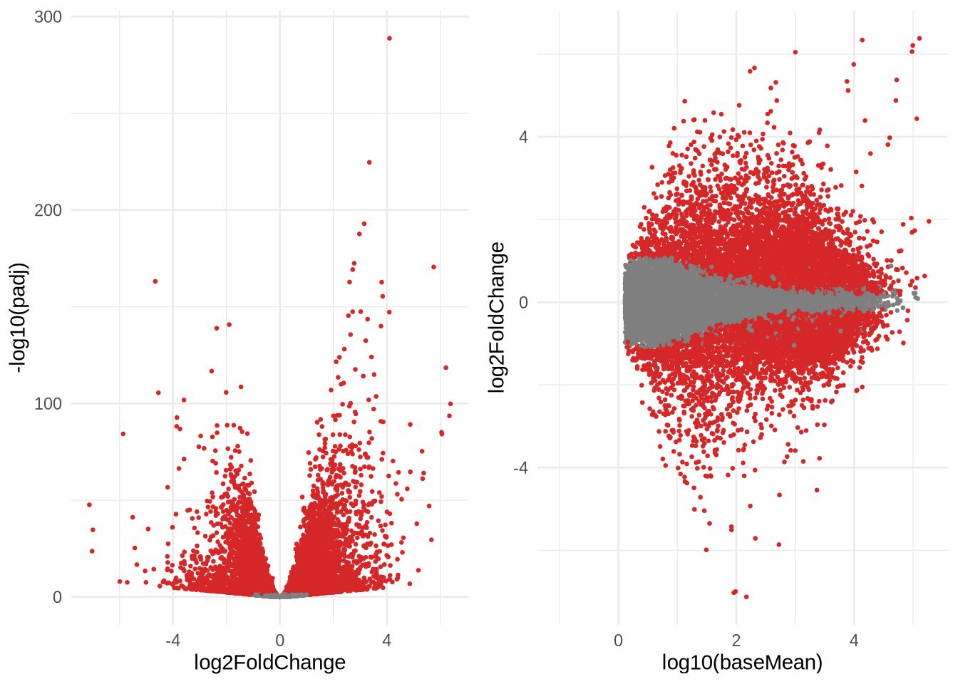
b. Likelihood ratio test
DESeq2 also offers the Likelihood Ratio Test (LRT) as an alternative to Wald test when evaluating expression change across more than two levels. Rather than evaluating whether a gene’s expression is up- or down-regulated in one group compared to another, it identifies genes whose residual variance decreases significantly upon inclusion of a specified set of covariates. There is no need for contrasts since we are not making a pair-wise comparison. The LRT always compares a ‘full’ model (with all of the covariates) to a ‘reduced’ model (with a number of covariates removed). Note thus that the reduced model is always nested with respect to the full model.
One can use an LRT to test for one factor too (which asymptotically would be equivalent to a wald test), but for the sake of illustration (and why the LRT is useful) we can identify genes that are sensitive to any treatment, or even both. Note that we have DMSO, TG & AMIL, and thus would need two contrasts to identify genes changing with respect to the base level. With the LRT we can drop both ‘condition’ coefficients in the reduced model.
The LRT is comparing the ‘full’ model to the ‘reduced’ model to identify significant genes. The p-values are determined solely by the difference in deviance between the ‘full’ and the ‘reduced’ model formula (not the log2 fold changes).
dds_lrt_example <- dds
design(dds_lrt_example) <- ~celltype + condition
dds_lrt_example <- DESeq(dds_lrt_example)
print(design(dds_lrt_example))
## ~celltype + conditionprint(resultsNames(dds_lrt_example))## [1] "Intercept" "celltype_JJ_vs_BM" "condition_DMSO_vs_AMIL"
## [4] "condition_TG_vs_AMIL"dds_lrt <- DESeq(dds_lrt_example, test="LRT", reduced = ~celltype)
res_lrt <- results(dds_lrt)
head(res_lrt)## log2 fold change (MLE): condition TG vs AMIL
## LRT p-value: '~ celltype + condition' vs '~ celltype'
## DataFrame with 6 rows and 6 columns
## baseMean log2FoldChange lfcSE stat pvalue
## <numeric> <numeric> <numeric> <numeric> <numeric>
## ENSG00000000419 2285.01560 -0.280813 0.1599274 11.01680 4.05258e-03
## ENSG00000000457 775.42002 0.449928 0.0783874 35.43819 2.01695e-08
## ENSG00000000460 1300.43696 0.791716 0.0835904 139.66593 4.69817e-31
## ENSG00000000938 2.45443 0.739592 0.7879720 1.64233 4.39919e-01
## ENSG00000000971 1626.92877 0.189846 0.1134560 6.35776 4.16323e-02
## ENSG00000001036 992.80507 -1.118897 0.2469728 19.37905 6.19289e-05
## padj
## <numeric>
## ENSG00000000419 7.52527e-03
## ENSG00000000457 8.12254e-08
## ENSG00000000460 7.06354e-30
## ENSG00000000938 5.11609e-01
## ENSG00000000971 6.33396e-02
## ENSG00000001036 1.56764e-04Columns relevant to the LRT test:
- baseMean: mean of normalized counts for all samples
- stat: the difference in deviance between the reduced model and the full model
- pvalue: the stat value is compared to a chi-squared distribution to generate a pvalue
- padj: BH adjusted p-values
Reminder: Note that the l2FC/lfcSE is again from our last coefficient ! (and thus doesn’t tell us anything in this case).
sig_res_lrt <- res_lrt %>% data.frame()  %>% drop_na() %>% dplyr::filter(padj < 0.05) %>% arrange(padj)
nrow(sig_res_lrt)
## [1] 14441pheatmap(counts(dds, normalized=TRUE)[sig_res_lrt %>% rownames(),],
cluster_rows = T,
show_rownames = F,
border_color = NA,
fontsize = 10,
scale = "row",
fontsize_row = 10,
height = 20)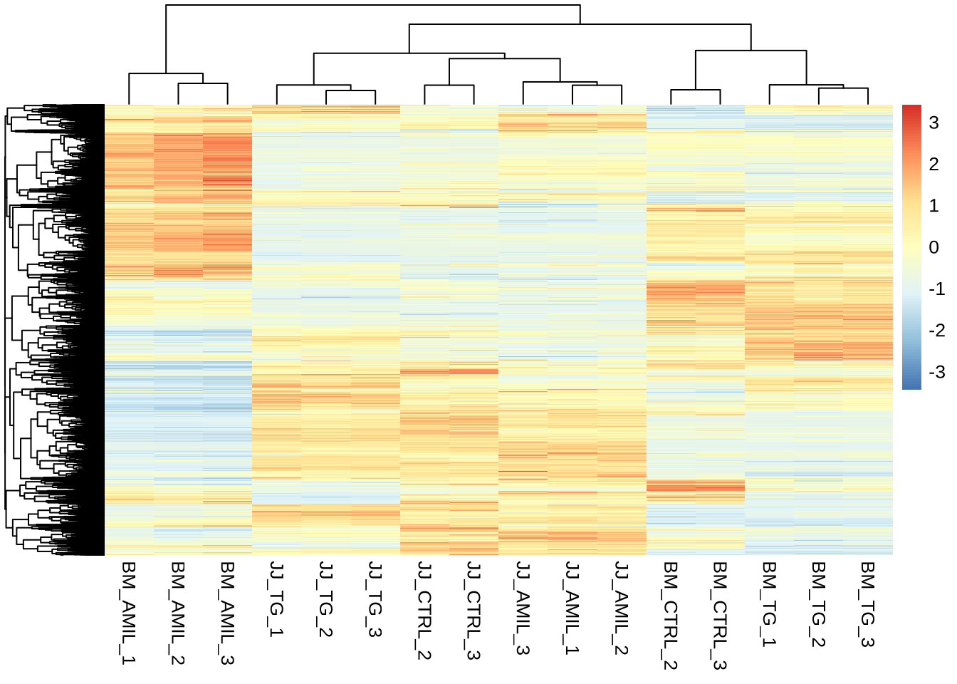
pheatmap(counts(dds, normalized=TRUE)[sig_res_lrt %>% rownames(),],
         cluster_rows = T,
         kmeans_k = 10,
         show_rownames = F,
         border_color = NA,
         fontsize = 10,
         scale = "row",
         fontsize_row = 10,
         height = 20)
c. Back to square one.
We now have an idea on how we can extract pair-wise comparisons from a multi-factor DESeq2 analysis, and we got a primer on comparisons beyond pair-wise comparisons. What now ? Let’s try to extract something biologically meaningful from the data.
Remember that all the data + metadata + design are available in our DESeq object (dds)
Reminder: attributes(dds)
… our factors:
colData(dds)$celltype## [1] BM BM BM BM BM JJ JJ JJ JJ JJ BM BM BM JJ JJ JJ
## Levels: BM JJcolData(dds)$condition## [1] DMSO DMSO AMIL AMIL AMIL DMSO DMSO AMIL AMIL AMIL TG TG TG TG TG
## [16] TG
## Levels: AMIL DMSO TG… our design
design(dds)## ~celltype + condition + celltype:conditionPoll 3.4: Is there a difference in specifying ~celltype*condition and ~celltype + condition + celltype:condition ?
Reminder: This is in essence a drug repurposing study.
A couple of other relevant notes:
- BM and JJ are two cell lines generated from multiple myeloma patients.
- (alternative) splicing is affected in this cancer.
- TG003 is a drug commonly used in this disease (clk1 kinase inhibitor)
- Amiloride is an old drug (diuretic) that is hypothesized to be a good candidate for repurposing in multiple myeloma.
d. amiloride vs TG
Let’s start by assessing the difference between amiloride treated cells and TG treated cells.
Remember our coefficients:
resultsNames(dds)## [1] "Intercept" "celltype_JJ_vs_BM"
## [3] "condition_DMSO_vs_AMIL" "condition_TG_vs_AMIL"
## [5] "celltypeJJ.conditionDMSO" "celltypeJJ.conditionTG"And remember: contrasts can be specified in a number of ways.
- Character vector with three elements: c(factor1, level1, level2) !
- A list with 2 coefficients
- A numeric vector with a value for each coefficient
Extract TG vs AMIL:
TGvAMIL <- lfcShrink(dds, contrast = c('condition', 'TG', 'AMIL'), type="ashr")
head( TGvAMIL %>% data.frame() )
# or
TGvAMIL <- lfcShrink(dds, contrast = c(0,0,0,1,0,0), type="ashr")
head( TGvAMIL %>% data.frame() )! Make sure you have the ‘TGvAMIL’ results object.
Poll 3.5: Given our contrast c(‘condition’, ‘TG’, ‘AMIL’), what would a (significant) positive foldchange correspond to ?
colData(dds)$celltype## [1] BM BM BM BM BM JJ JJ JJ JJ JJ BM BM BM JJ JJ JJ
## Levels: BM JJFor celltype JJ, things are a bit more tricky. We cannot use the c(factor1, level1, level2) contrast (since BM is our baseline!), and the coefficient we are interested in is actually not in resultsNames (it’s a combination of AMIL-TG + the interaction term TG-JJ). We thus have to specify the numerical vector or use a list. You can build these manually (which is error prone), but there is a trick that could make our life easier. This is based on the model matrix:
pheatmap(model.matrix(design(dds), colData(dds)),
         cluster_cols = FALSE,
         cluster_rows = FALSE)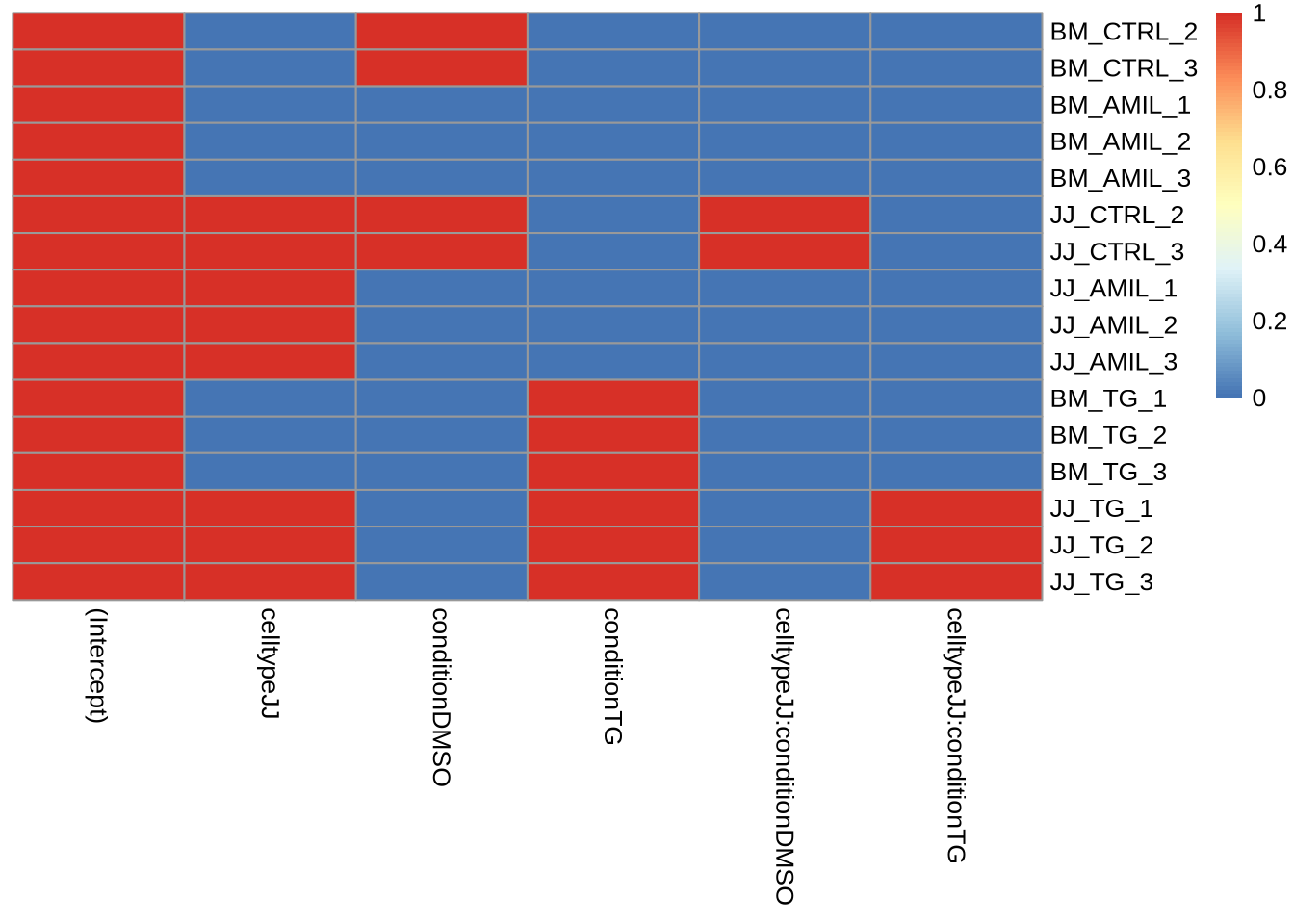
The workflow is as follows:
- Get the model matrix.
- Get the colMeans of a subset of the matrix for each group of interest.
- Subtract the group vectors from each other.
- graduate summa cum laude
The convenient part about this method is that rather than thinking about the coefficients, you think about factor levels. A more elaborate tutorial can be found here
! Note that we also could rerun DESeq with the appropriate factor re-leveled, though this is cumbersome
We’d like to see the difference between condition TG and AMIL in cellType JJ. (Note that based on our factor levels, this is essentially coefficient TG_vs_AMIL + interactionJJ:TG)
mod_mat <- model.matrix(design(dds), colData(dds))

# Remember we'd like to compare TG treatment with AMIL treatment in JJ cells.
JJ_TG <- colMeans(mod_mat[dds$celltype == 'JJ' & dds$condition == "TG",])
JJ_AMIL <- colMeans(mod_mat[dds$celltype == 'JJ' & dds$condition == "AMIL",])

print(JJ_TG - JJ_AMIL)
## (Intercept) celltypeJJ conditionDMSO
## 0 0 0
## conditionTG celltypeJJ:conditionDMSO celltypeJJ:conditionTG
## 1 0 1TGvAMIL_JJ <- lfcShrink(dds, contrast = JJ_TG - JJ_AMIL, type="ashr")TGvAMIL_JJ_2 <- lfcShrink(dds, contrast = list(c("condition_TG_vs_AMIL", "celltypeJJ.conditionTG")), type="ashr")## using 'ashr' for LFC shrinkage. If used in published research, please cite:
## Stephens, M. (2016) False discovery rates: a new deal. Biostatistics, 18:2.
## https://doi.org/10.1093/biostatistics/kxw041TGvAMIL_JJ %>% head()## log2 fold change (MMSE): 0,0,0,+1,0,+1
## Wald test p-value: 0,0,0,+1,0,+1
## DataFrame with 6 rows and 5 columns
## baseMean log2FoldChange lfcSE pvalue padj
## <numeric> <numeric> <numeric> <numeric> <numeric>
## ENSG00000000419 2285.01560 -0.133156 0.1792227 4.14521e-01 5.60917e-01
## ENSG00000000457 775.42002 0.296568 0.0914493 8.82329e-04 2.60712e-03
## ENSG00000000460 1300.43696 0.677672 0.1097990 1.37967e-10 1.00379e-09
## ENSG00000000938 2.45443 -0.134278 0.5047156 5.58789e-01 7.02617e-01
## ENSG00000000971 1626.92877 0.179904 0.0874474 3.54027e-02 7.35916e-02
## ENSG00000001036 992.80507 -0.298974 0.0860456 3.80931e-04 1.19393e-03TGvAMIL_JJ_2 %>% head()## log2 fold change (MMSE): condition_TG_vs_AMIL+celltypeJJ.conditionTG effect
## Wald test p-value: condition_TG_vs_AMIL+celltypeJJ.conditionTG effect
## DataFrame with 6 rows and 5 columns
## baseMean log2FoldChange lfcSE pvalue padj
## <numeric> <numeric> <numeric> <numeric> <numeric>
## ENSG00000000419 2285.01560 -0.133156 0.1792227 4.14521e-01 5.60917e-01
## ENSG00000000457 775.42002 0.296568 0.0914493 8.82329e-04 2.60712e-03
## ENSG00000000460 1300.43696 0.677672 0.1097990 1.37967e-10 1.00379e-09
## ENSG00000000938 2.45443 -0.134278 0.5047156 5.58789e-01 7.02617e-01
## ENSG00000000971 1626.92877 0.179904 0.0874474 3.54027e-02 7.35916e-02
## ENSG00000001036 992.80507 -0.298974 0.0860456 3.80931e-04 1.19393e-03! Make sure you have the ‘TGvAMIL_JJ’ results object.
! Cave ! The colMeans trick should ONLY be used when you have BALANCED designs. If the number of samples differes between the groups you want to compare, this could lead to a WRONG contrast.
So in general (and this goes beyond RNA-seq analysis), think about what you are doing and if it makes sense.
e. Clean & Annotate
- we only have transcript IDs, not actual gene names.
- Commonly used package to convert between them is biomaRt.
- Alternatively (without API/internet) is org.Hs.eg.db package.
Reminder: Hs -> Homo Sapiens. As you probably guessed, for most model organisms there is a package like this (mm, sp, …) ). Since the data is processed with GRCh37, we will use the following database: “EnsDb.Hsapiens.v75”. Which is already rather outdated at this time. Note that this should match the reference used to create the count matrix !
In our case we can use:
ensembldb::select(EnsDb.Hsapiens.v75, keys= ensemble, keytype = “GENEID”, columns = c(“SYMBOL”,“GENEID”))
Reminder: Some function between ensembldb (part of EnsDb.Hsapiens.v79) and dplyr overlap. Explicitly state the library when calling them to avoid errors.
Remember. With our contrast juggling we have 2 results objects (‘Large DESeqResults’).
TGvAMIL (for BM cells). TGvAMIL_JJ (for JJ cells).
Task: Clean our results classes (TGvAMIL & TGvAMIL_JJ) (15 min)
- convert the results object into a dataframe
- remove the na values from the dataframe
- Sort the dataframe by adjusted p value
- Include the gene names (== ‘SYMBOL’) as a ‘gene_symbol’ column in the dataframe
- if you are feeling brave, you can wrap these operations in a function!
Hint for the symbols, this is how ensembldb::select works (to return a SYMBOL - GENEID mapping) Hint2: The accessions (==GENEIDS) were stored as rownames in our count matrix. Where are they in the dds object ?
cleanDF <- function(RESobj){
  RESdf <- data.frame(RESobj) %>%
    drop_na() %>%
    arrange(padj)
  RESdf$gene_symbol <- ensembldb::select(EnsDb.Hsapiens.v75, keys = rownames(RESdf),
                                         keytype = "GENEID", columns = c("SYMBOL", "GENEID"))$SYMBOL
  return(RESdf)
}

TGvAMIL_JJ_cleaned <- cleanDF(TGvAMIL_JJ)
TGvAMIL_BM_cleaned <- cleanDF(TGvAMIL)
# Plot Zscores for top20 hits.
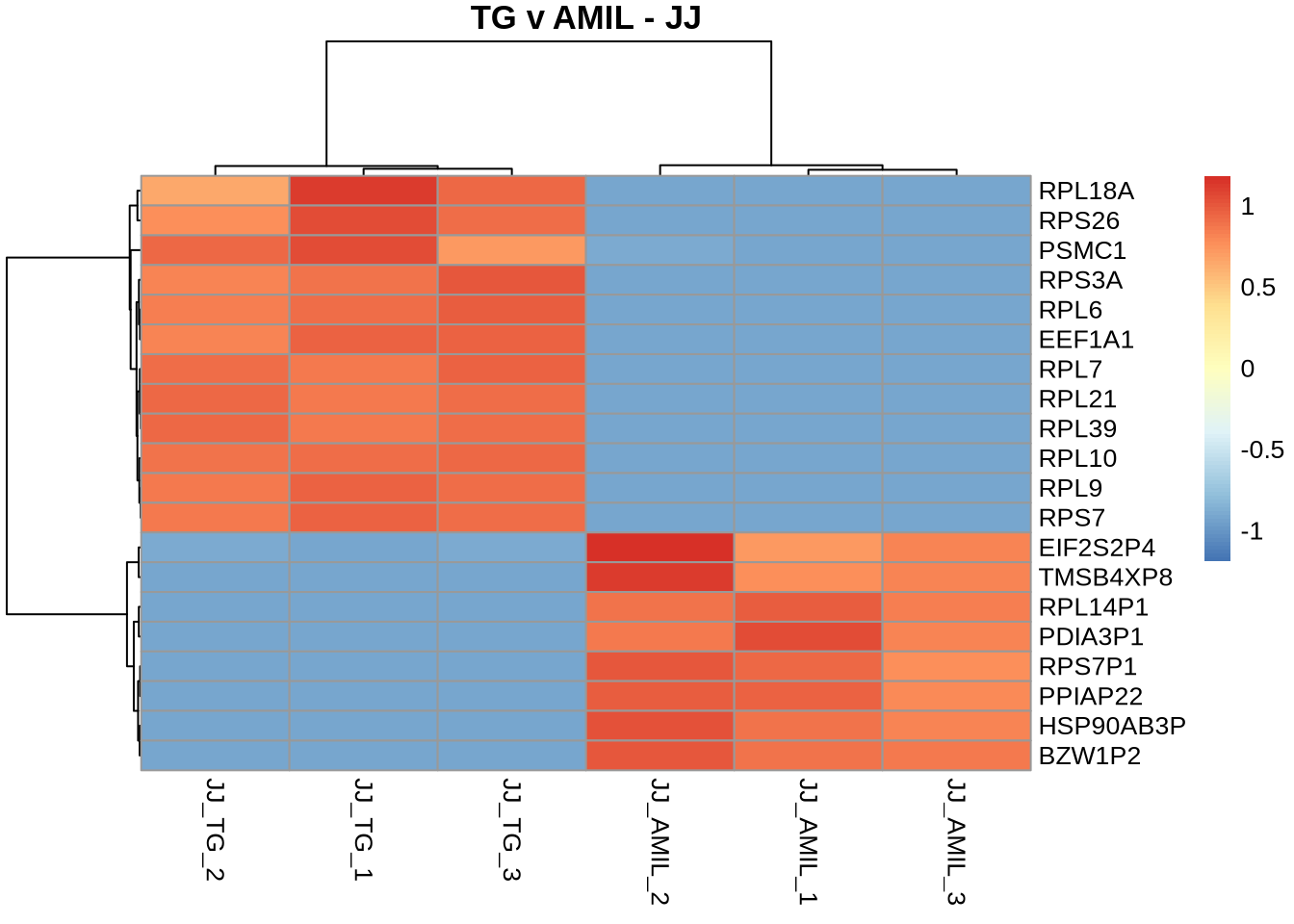
pheatmap(
counts(dds, normalized=TRUE)[TGvAMIL_JJ_cleaned %>% rownames %>% head(20), c(8,9,10,14,15,16)],
scale = 'row',
main='TG v AMIL - JJ',
labels_row = TGvAMIL_JJ_cleaned %>% head(20) %>% pull('gene_symbol')
)
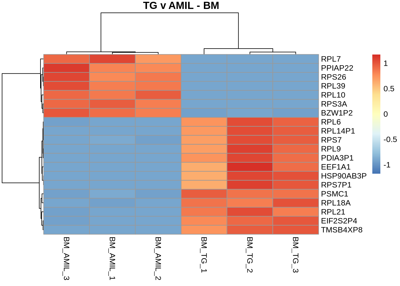
pheatmap(
  counts(dds, normalized=TRUE)[TGvAMIL_BM_cleaned %>% rownames %>% head(20), c(3,4,5,11,12,13)],
  scale = 'row',
  main='TG v AMIL - BM',
  labels_row = TGvAMIL_JJ_cleaned %>% head(20) %>% pull('gene_symbol')
)
To look at the overlaps:
upsetList <- list(
  "BM - Up" = TGvAMIL_BM_cleaned %>% dplyr::filter(padj < 0.05, log2FoldChange > 2) %>% rownames(),
  "BM - Down" = TGvAMIL_BM_cleaned %>% dplyr::filter(padj < 0.05, log2FoldChange < -2) %>% rownames(),
  "JJ - Up" = TGvAMIL_JJ_cleaned %>% dplyr::filter(padj < 0.05, log2FoldChange > 2) %>% rownames(),
  "JJ - Down" = TGvAMIL_JJ_cleaned %>% dplyr::filter(padj < 0.05, log2FoldChange < -2) %>% rownames()
  )

upset(fromList(upsetList), order.by = "freq")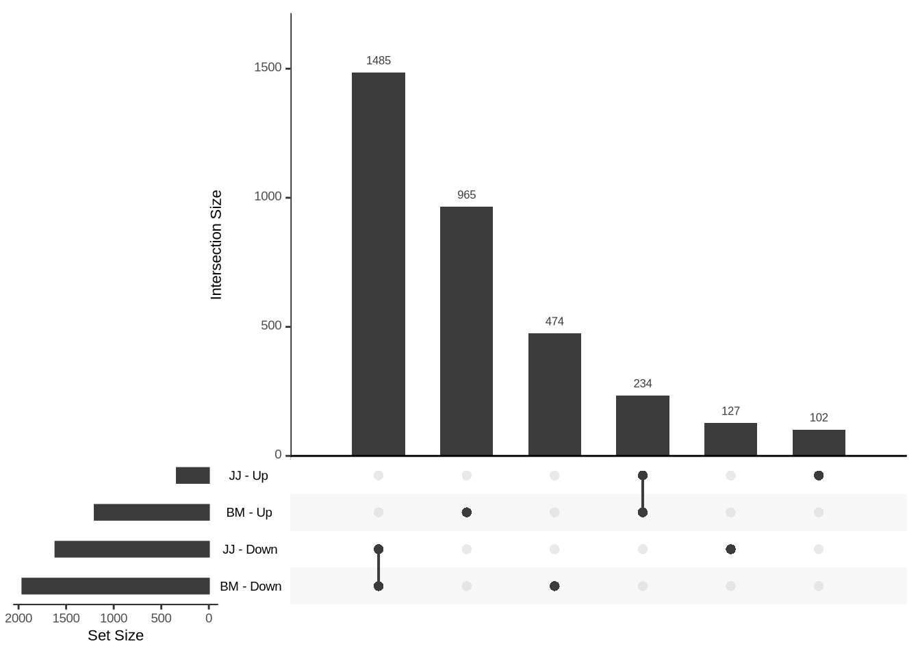
f. Apoptosis & Spliceosome
Finally, look at two specific geneSets. - genes involved in splicing - genes involved in apoptosis
Note that we will read in the txt files as a vector (with gene symbols).
keggf <- 'data/genesets/KEGG_apoptosis.txt'
splicef <- 'data/genesets/KEGG_spliceosome.txt'

kegg_apoptosis <- read_tsv(file=keggf, col_names = FALSE)
kegg_apoptosis <- kegg_apoptosis$X1

kegg_spliceosome <- read_tsv(file=splicef, col_names = FALSE)
kegg_spliceosome <- kegg_spliceosome$X1
kegg_spliceosome %>% head()
## [1] "ACIN1" "ALYREF" "AQR" "BCAS2" "BUD31" "CCDC12"retIDsfromSymbolList <- function(df, symbols){
return(df %>% subset(gene_symbol %in% symbols) %>% subset(padj < 0.05) %>% rownames())
}
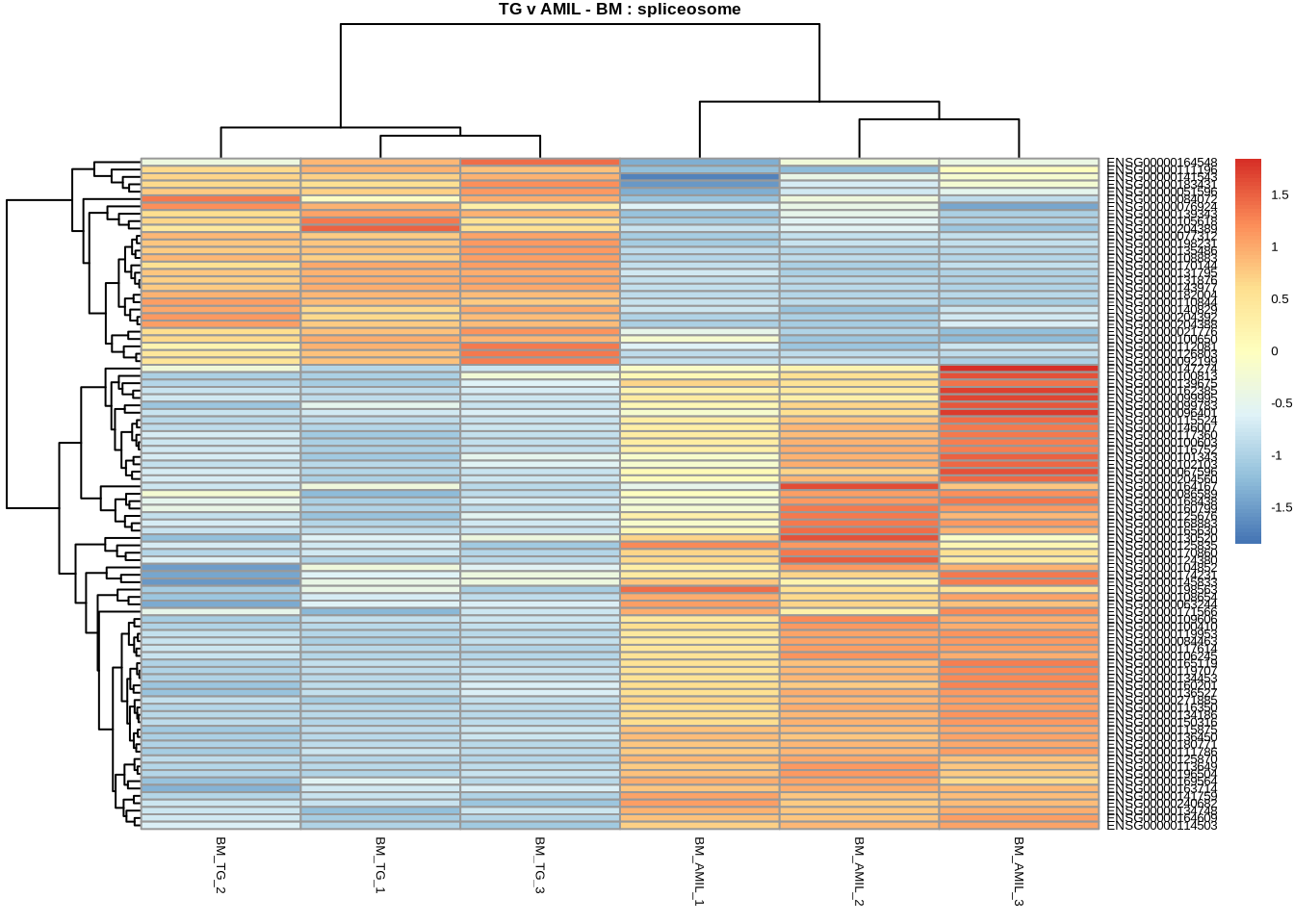
# spliceosome
pheatmap(
counts(dds, normalized=TRUE)[
retIDsfromSymbolList(TGvAMIL_BM_cleaned, kegg_spliceosome),
c(3,4,5,11,12,13)
],
scale = 'row',
main='TG v AMIL - BM : spliceosome',
fontsize=5
)
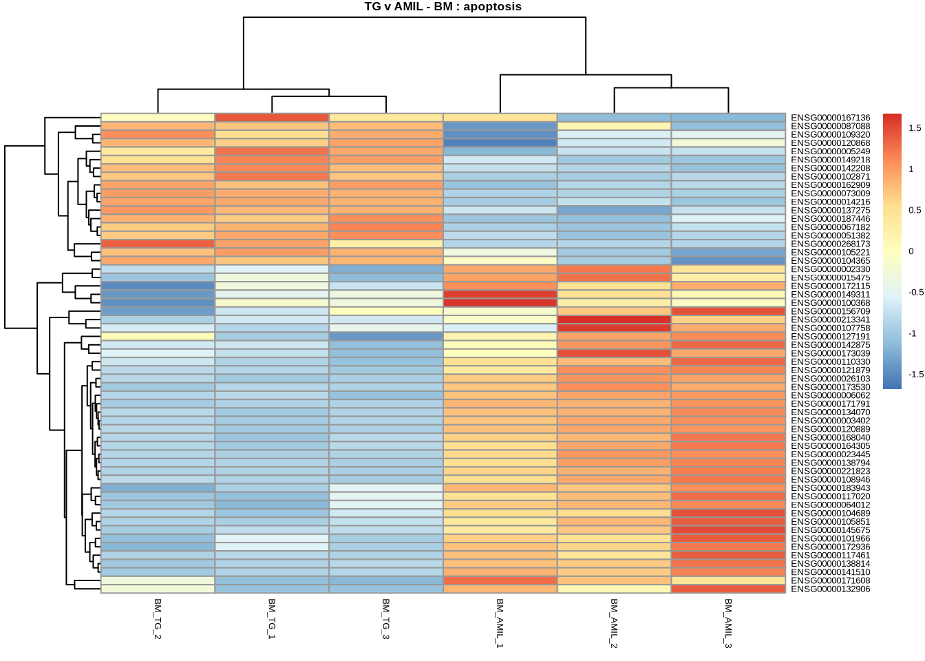
# Apoptosis

pheatmap(
  counts(dds, normalized=TRUE)[
    retIDsfromSymbolList(TGvAMIL_BM_cleaned, kegg_apoptosis),
    c(3,4,5,11,12,13)
  ],
  scale = 'row',
  main='TG v AMIL - BM : apoptosis',
  fontsize=5
)
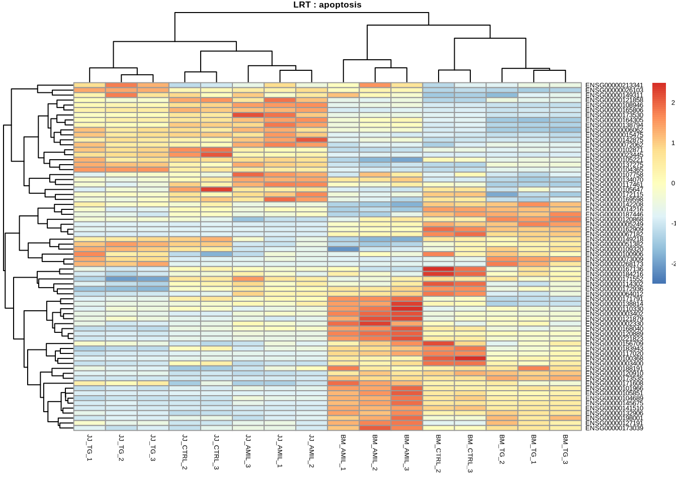
g. LRT
Finally, let’s look at the treatment factor using LRT. For this we’ll use ~celltype as the reduced model.
dds_lrt <- DESeq(dds, test="LRT", reduced = ~celltype)
res_lrt <- results(dds_lrt)
Now let’s clean the dataframe, write out the results in a tsv file, and redo our heatmap exercise for the pathways.
res_lrt_clean <- cleanDF(res_lrt)
res_lrt_clean
# Write out results in a tsv file.
write.table(res_lrt_clean, file="lrtResults.tsv", quote = FALSE, sep = "\t")
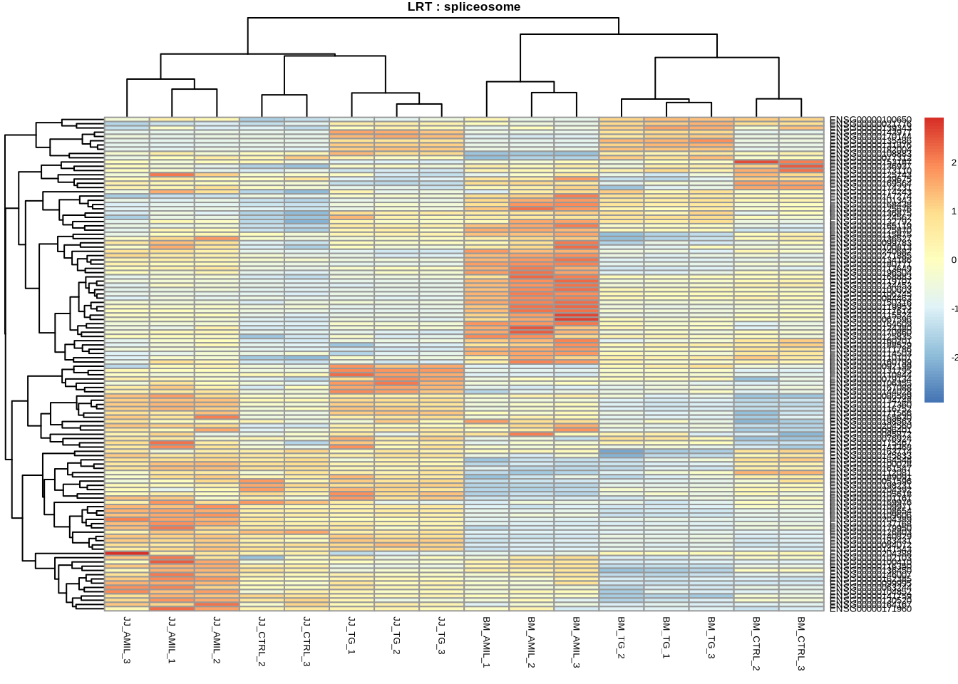
# spliceosome
pheatmap(
counts(dds, normalized=TRUE)[
retIDsfromSymbolList(res_lrt_clean, kegg_spliceosome),
],
scale = 'row',
main='LRT : spliceosome',
fontsize=5
)
# Apoptosis
pheatmap(
  counts(dds, normalized=TRUE)[
    retIDsfromSymbolList(res_lrt_clean, kegg_apoptosis),
  ],
  scale = 'row',
  main='LRT : apoptosis',
  fontsize=5
)