Differential Expression Analyses
Setup
# .libPaths(new = "/scratch/local/rseurat/pkg-lib-4.2.3")

suppressMessages({
  library(tidyverse)
  library(Seurat)
})


set.seed(8211673)

knitr::opts_chunk$set(echo = TRUE, format = TRUE, out.width = "100%")


options(parallelly.fork.enable = FALSE,
        future.globals.maxSize = 8 * 1024 ^ 2 * 1000)

plan("multicore", workers = 8)
## work directory: /home/runner/work/Rseurat/Rseurat/rmd## library path(s): /home/runner/micromamba/envs/Rseurat/lib/R/libraryLoad Data
We’ll be working with the data from Day 1 (“First steps”), let’s quickly re-load and re-process again:
pbmc <- Read10X(data.dir = "./datasets/filtered_gene_bc_matrices/hg19/") %>%
  CreateSeuratObject(counts = ., project = "pbmc3k", min.cells = 3, min.features = 200)

pbmc[["percent.mt"]] <- PercentageFeatureSet(pbmc, pattern = "^MT-")

pbmc <- subset(pbmc, subset = nFeature_RNA > 200 & nFeature_RNA < 2500 & percent.mt < 5)

pbmc <- NormalizeData(pbmc, verbose = FALSE)

pbmc <- FindVariableFeatures(pbmc, verbose = FALSE)

pbmc <- ScaleData(pbmc, features = rownames(pbmc), verbose = FALSE)

pbmc <- RunPCA(pbmc, features = VariableFeatures(pbmc), verbose = FALSE)

pbmc <- FindNeighbors(pbmc, dims = seq_len(10), verbose = FALSE)

pbmc <- FindClusters(pbmc, resolution = 0.5, verbose = FALSE)

pbmc <- RunUMAP(pbmc, dims = seq_len(10), verbose = FALSE)
Searching for Markers
Having identified (and visualized) clusters of cells we want to learn about the specific genes under differential expression.
We will focus on how to derive marker genes for any
given groups of cells. To this end, Seurat has different convenient
functions that run Differential Expression (DE) tests.
One such function, and the main one is FindMarkers(). Among
other parameters, it takes:
ident.1, andident.2: typically these denote specific cluster numbers (“identities”) of cells, but any other annotation from the metadata will work as well.test.use: select from a wide range of statistical models and/ or methodologies (we use “MAST”)
MAST controls for the proportion of genes detected in each
cell, this acts as a proxy for both technical (e.g., dropout,
amplification efficiency) and biological factors (e.g., cell volume and
extrinsic factors other than treatment of interest) that globally
influence gene expression. It is a two-part generalized linear model
that simultaneously models the rate of expression over the background of
various transcripts, and the positive expression mean. Another popular
option is DESeq2, with plenty
of caveats that the Seurat authors may have addressed.
Let’s do a comparison between cells that were assigned to either cluster 1 or 2.
markers1v2 <- FindMarkers(
  object = pbmc,
  test.use = "MAST",
  ident.1 = 1,
  ident.2 = 2,
  verbose = FALSE
)
##
## Done!## Combining coefficients and standard errors## Calculating log-fold changes## Calculating likelihood ratio tests## Refitting on reduced model...##
## Done!The resulting object is a data frame with the following columns:
p_val: p-value (unadjusted!)avg_log2FC: log fold-change of the average expression between the two groups. Positive values indicate that the feature is more highly expressed in the first group.pct.1: The percentage of cells where the feature is detected in the first grouppct.2: The percentage of cells where the feature is detected in the second groupp_val_adj: Adjusted p-value, based on Bonferroni correction using all features in the dataset.
You may inspect the results with either View() or
head().
🧭✨ Polls:
Given that genes used for clustering are the same genes tested for differential expression, Would you interpret the (adjusted) p-values without concerns?
Which marker gene is the most expressed in cluster 1 when comparing it to cluster 2?
What would happen if we used
ident.1 = 2, andident.2 = 1instead?
Notice:
- Regarding the ‘double-dipping’ issue asked in the first question above, there’s this statistical method but it’s not implemented (yet, afaik.)
- If
ident.2=NULL(default), thenFindMarkers()will run a test between the groupident.1and all other cells - You may also use a vector (e.g.
c(1,3)) asident.2to compare against all the cells of clusters one and three, pooled together. - to increase the speed and relevance of marker discovery, Seurat
allows for pre-filtering of features or cells. For example, genes that
are very infrequently detected in either group of cells, or genes that
are expressed at similar average levels, are unlikely to be
differentially expressed, so we can exclude those:
?FindMarkers
There are different flavors of these Find* functions.
It’s important to get to know them!
FindMarkerswill find markers between two different identity groups - you have to specify both identity groups. This is useful for comparing the differences between two specific groups.FindAllMarkerswill find markers differentially expressed in each identity group by comparing it to all of the others - you don’t have to manually define anything. Note that markers may bleed over between closely-related groups - they are not forced to be specific to only one group.FindConservedMarkerswill find markers that are conserved between two groups of cells, across different conditions (for example, a treated and control).FindConservedMarkershas a mandatory argument, the grouping variable (grouping.var), and the function is used to compare across groups (conditions), it will combine p-values of runningFindMarkersfor the two groups of cells (idents), in each condition. It means they are differentially expressed compared to other groups in the respective conditions, but have differential expression between the those two groups across the conditions.
Graphical Exploration
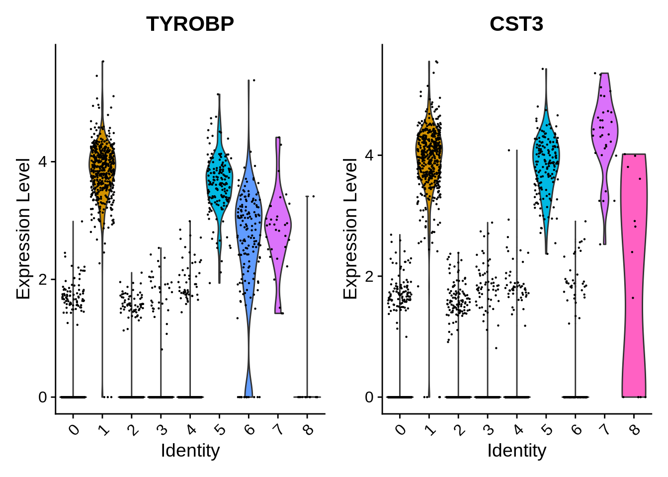
Seurat includes several tools for visualizing marker expression.
VlnPlot and RidgePlot show the probability
density distributions of expression values across clusters, and
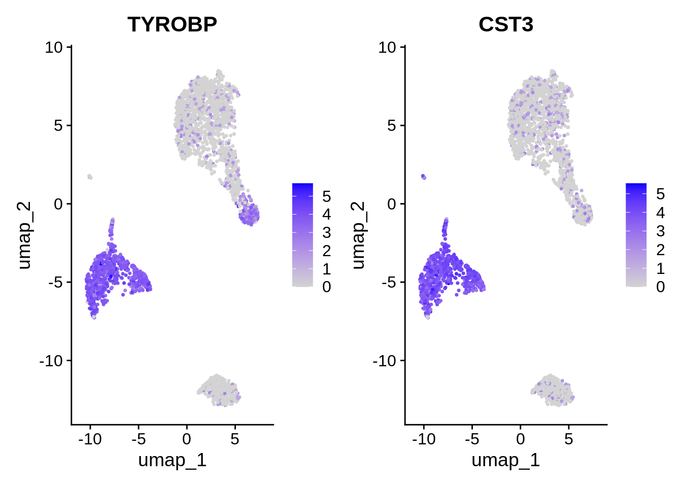
FeaturePlot() visualizes feature expression in a reduction
(e.g. PCA, t-SNE, or UMAP). The latter is equivalent to
DimPlot.
⌨🔥 Exercise: Draw a RidgePlot with the vector
feats.
Markers Per Cluster (between)
What are the differences between clusters? disregarding any other metadata (cell-cycle, treatments, groups, etc). Let’s compare 1 vs all, 2 vs all, … etc.
For computational efficiency we’ll use pbmc_small which
is a downsampled PBMC3K data set bundled with Seurat. (Yes, it won’t
appear in your Global Environment but it’s ready to be loaded upon
execution of code.)
markers.between.clusters <- FindAllMarkers(
  pbmc_small,
  test.use = "MAST",
  logfc.threshold = 0.125,
  min.pct = 0.05,
  only.pos = TRUE,
  densify = TRUE
)
## Calculating cluster 0##
## Done!## Combining coefficients and standard errors## Calculating log-fold changes## Calculating likelihood ratio tests## Refitting on reduced model...##
## Done!## Calculating cluster 1##
## Done!## Combining coefficients and standard errors## Calculating log-fold changes## Calculating likelihood ratio tests## Refitting on reduced model...##
## Done!## Calculating cluster 2##
## Done!## Combining coefficients and standard errors## Calculating log-fold changes## Calculating likelihood ratio tests## Refitting on reduced model...##
## Done!## p_val avg_log2FC pct.1 pct.2 p_val_adj cluster gene
## GNLY 3.650213e-06 7.5951567 0.444 0.068 8.395490e-04 0 GNLY
## CCL5 7.316150e-06 2.1637570 0.667 0.273 1.682714e-03 0 CCL5
## CD7 1.747043e-05 3.8815815 0.528 0.091 4.018199e-03 0 CD7
## LAMP1 8.331300e-05 4.2754193 0.444 0.068 1.916199e-02 0 LAMP1
## NKG7 1.040648e-04 2.0463041 0.472 0.409 2.393491e-02 0 NKG7
## TUBB1 1.277014e-04 11.7032356 0.250 0.000 2.937131e-02 0 TUBB1
## GP9 1.277014e-04 10.9796850 0.250 0.000 2.937131e-02 0 GP9
## NGFRAP1 1.277014e-04 10.3900756 0.250 0.000 2.937131e-02 0 NGFRAP1
## GZMA 2.841378e-04 2.4750157 0.444 0.068 6.535170e-02 0 GZMA
## NOSIP 2.978655e-04 3.1107859 0.444 0.250 6.850907e-02 0 NOSIP
## AKR1C3 3.461924e-04 10.3326298 0.222 0.000 7.962426e-02 0 AKR1C3
## PGRMC1 3.461924e-04 10.1143303 0.222 0.000 7.962426e-02 0 PGRMC1
## LCK 4.086765e-04 2.7174842 0.500 0.114 9.399559e-02 0 LCK
## PPBP 5.727274e-04 6.2210236 0.278 0.068 1.317273e-01 0 PPBP
## PF4 7.269306e-04 7.8762665 0.250 0.023 1.671940e-01 0 PF4
## PRF1 8.869645e-04 2.4884769 0.417 0.091 2.040018e-01 0 PRF1
## TMEM40 9.229981e-04 9.7113490 0.194 0.000 2.122896e-01 0 TMEM40
## GZMB 9.883116e-04 4.5344157 0.333 0.091 2.273117e-01 0 GZMB
## CST7 1.151716e-03 2.3576102 0.472 0.182 2.648947e-01 0 CST7
## CD247 1.321001e-03 3.1919811 0.389 0.068 3.038302e-01 0 CD247
## IL32 1.357829e-03 2.6835667 0.444 0.182 3.123006e-01 0 IL32
## GNG11 1.624489e-03 6.8127586 0.250 0.023 3.736324e-01 0 GNG11
## GZMM 1.692823e-03 2.2558215 0.417 0.091 3.893494e-01 0 GZMM
## ACAP1 1.744305e-03 4.9623836 0.306 0.045 4.011901e-01 0 ACAP1
## XBP1 2.004571e-03 2.6445880 0.444 0.159 4.610513e-01 0 XBP1
## KLRD1 2.113001e-03 4.9323956 0.278 0.023 4.859903e-01 0 KLRD1
## GIMAP1 2.116378e-03 2.9412718 0.417 0.273 4.867669e-01 0 GIMAP1
## CD3D 2.297727e-03 1.4719637 0.472 0.136 5.284773e-01 0 CD3D
## PTCRA 2.426135e-03 10.2639307 0.167 0.000 5.580111e-01 0 PTCRA
## GPX1 2.811945e-03 1.1142613 0.556 0.750 6.467474e-01 0 GPX1
## SDPR 2.893784e-03 5.4636858 0.250 0.045 6.655703e-01 0 SDPR
## NCOA4 3.497782e-03 3.5144647 0.306 0.159 8.044898e-01 0 NCOA4
## TPM4 3.929968e-03 2.3114013 0.444 0.273 9.038925e-01 0 TPM4
## CLU 4.048166e-03 5.6000850 0.250 0.023 9.310781e-01 0 CLU
## IL7R 4.607904e-03 3.0584481 0.389 0.295 1.000000e+00 0 IL7R
## CD3E 5.195127e-03 2.5655245 0.444 0.205 1.000000e+00 0 CD3E
## CD9 5.900192e-03 4.7767245 0.250 0.023 1.000000e+00 0 CD9
## GZMH 6.272982e-03 3.5948085 0.250 0.023 1.000000e+00 0 GZMH
## SAFB2 6.306739e-03 9.5098713 0.139 0.000 1.000000e+00 0 SAFB2
## RARRES3 7.019218e-03 1.8186318 0.528 0.250 1.000000e+00 0 RARRES3
## TALDO1 8.686875e-03 1.3435273 0.389 0.591 1.000000e+00 0 TALDO1
## EIF4A2 8.935622e-03 1.6124755 0.556 0.477 1.000000e+00 0 EIF4A2
## CA2 9.077357e-03 6.0702617 0.222 0.023 1.000000e+00 0 CA2
## S100A8 2.847665e-15 6.5990076 0.960 0.091 6.549630e-13 1 S100A8
## TYMP 6.288233e-14 3.2888895 1.000 0.164 1.446294e-11 1 TYMP
## S100A9 2.601646e-12 5.5250920 0.880 0.164 5.983786e-10 1 S100A9
## LYZ 1.144613e-11 3.0454906 1.000 0.473 2.632609e-09 1 LYZ
## CST3 1.553266e-11 2.3777356 1.000 0.327 3.572511e-09 1 CST3
## AIF1 7.395409e-11 2.4677179 1.000 0.273 1.700944e-08 1 AIF1
## LST1 9.019583e-11 2.6472667 0.960 0.200 2.074504e-08 1 LST1
## FCGRT 6.344380e-10 3.1859969 0.840 0.109 1.459207e-07 1 FCGRT
## TYROBP 1.643849e-09 2.1213129 1.000 0.382 3.780852e-07 1 TYROBP
## IFITM3 5.738102e-09 2.8154556 0.800 0.109 1.319763e-06 1 IFITM3
## S100A11 5.994495e-09 1.9813927 1.000 0.364 1.378734e-06 1 S100A11
## FCER1G 6.606599e-09 1.8630811 1.000 0.364 1.519518e-06 1 FCER1G
## FCN1 8.110417e-09 2.1945517 0.880 0.182 1.865396e-06 1 FCN1
## LGALS1 7.989746e-08 1.7459068 1.000 0.455 1.837642e-05 1 LGALS1
## GRN 1.225994e-07 2.3624897 0.760 0.127 2.819786e-05 1 GRN
## SERPINA1 1.851626e-07 3.2518562 0.720 0.109 4.258740e-05 1 SERPINA1
## PSAP 2.384511e-07 1.3275995 1.000 0.436 5.484375e-05 1 PSAP
## LGALS3 2.745689e-07 2.8289100 0.720 0.109 6.315085e-05 1 LGALS3
## SMCO4 3.460143e-07 3.7921864 0.520 0.018 7.958328e-05 1 SMCO4
## CD14 4.049172e-07 5.9141467 0.520 0.018 9.313095e-05 1 CD14
## BID 8.852004e-07 2.7681585 0.720 0.127 2.035961e-04 1 BID
## HLA-DRB1 1.370690e-06 0.3130038 0.880 0.345 3.152587e-04 1 HLA-DRB1
## CTSS 1.395130e-06 1.7891596 0.960 0.436 3.208800e-04 1 CTSS
## CTSB 1.564299e-06 3.1117200 0.680 0.109 3.597888e-04 1 CTSB
## FPR1 2.016368e-06 5.5241320 0.480 0.018 4.637647e-04 1 FPR1
## CFD 2.229943e-06 3.1204838 0.640 0.091 5.128869e-04 1 CFD
## IFI30 2.360071e-06 2.5132407 0.640 0.091 5.428164e-04 1 IFI30
## SAT1 3.559003e-06 1.6608880 1.000 0.582 8.185708e-04 1 SAT1
## HCK 3.584022e-06 3.0560240 0.560 0.055 8.243250e-04 1 HCK
## C5AR1 6.267039e-06 3.0270722 0.440 0.018 1.441419e-03 1 C5AR1
## IFI6 6.788620e-06 2.0224119 0.720 0.164 1.561383e-03 1 IFI6
## TSPO 7.931052e-06 2.1358314 0.880 0.364 1.824142e-03 1 TSPO
## HLA-DPB1 1.008014e-05 0.2075741 0.880 0.382 2.318431e-03 1 HLA-DPB1
## NUP214 1.280561e-05 3.0597800 0.480 0.036 2.945291e-03 1 NUP214
## CFP 1.393939e-05 2.2969910 0.680 0.145 3.206059e-03 1 CFP
## MS4A6A 1.500518e-05 3.2406748 0.520 0.055 3.451191e-03 1 MS4A6A
## CARD16 1.630711e-05 1.5611113 0.720 0.182 3.750636e-03 1 CARD16
## IL1B 2.142693e-05 4.8523958 0.480 0.055 4.928193e-03 1 IL1B
## LGALS2 2.796001e-05 3.0523244 0.600 0.109 6.430803e-03 1 LGALS2
## RNF130 3.381203e-05 3.3824278 0.560 0.091 7.776767e-03 1 RNF130
## GSTP1 3.837735e-05 1.4078657 0.880 0.364 8.826791e-03 1 GSTP1
## COTL1 5.787787e-05 1.5534206 0.960 0.545 1.331191e-02 1 COTL1
## RGS2 5.884770e-05 0.3660526 0.680 0.200 1.353497e-02 1 RGS2
## NFKBIA 7.026710e-05 1.1625780 0.880 0.382 1.616143e-02 1 NFKBIA
## HLA-DRB5 1.051939e-04 0.5602599 0.760 0.309 2.419460e-02 1 HLA-DRB5
## LINC00936 2.269283e-04 1.7851560 0.600 0.145 5.219351e-02 1 LINC00936
## ANXA2 3.441356e-04 0.6878531 0.840 0.400 7.915119e-02 1 ANXA2
## HLA-DPA1 3.742650e-04 0.8564766 0.840 0.382 8.608096e-02 1 HLA-DPA1
## ASGR1 5.485889e-04 5.4944900 0.320 0.018 1.261754e-01 1 ASGR1
## WARS 6.645957e-04 0.9639056 0.440 0.091 1.528570e-01 1 WARS
## BLVRA 7.687696e-04 1.5458200 0.560 0.145 1.768170e-01 1 BLVRA
## IL17RA 7.887600e-04 8.9743938 0.200 0.000 1.814148e-01 1 IL17RA
## LRRC25 1.672055e-03 1.5100103 0.440 0.091 3.845727e-01 1 LRRC25
## RBP7 1.928482e-03 2.8827067 0.280 0.018 4.435508e-01 1 RBP7
## CD68 2.086156e-03 2.1899000 0.520 0.145 4.798160e-01 1 CD68
## MPEG1 2.678808e-03 2.2679902 0.400 0.073 6.161257e-01 1 MPEG1
## HLA-DQA1 3.701779e-03 0.1700967 0.520 0.236 8.514091e-01 1 HLA-DQA1
## HLA-DMA 3.837196e-03 0.9162510 0.560 0.200 8.825551e-01 1 HLA-DMA
## VSTM1 7.460020e-03 4.3465859 0.240 0.018 1.000000e+00 1 VSTM1
## SCO2 8.968442e-03 2.8265606 0.320 0.055 1.000000e+00 1 SCO2
## HLA-DPB11 1.950378e-07 2.5347345 0.947 0.410 4.485870e-05 2 HLA-DPB1
## MS4A1 6.434726e-07 7.6239517 0.526 0.033 1.479987e-04 2 MS4A1
## HLA-DRA 1.218985e-06 2.6211073 0.895 0.623 2.803665e-04 2 HLA-DRA
## HLA-DQB1 1.444563e-06 3.0151024 0.789 0.246 3.322494e-04 2 HLA-DQB1
## HLA-DRB11 4.827866e-06 2.4070871 0.842 0.410 1.110409e-03 2 HLA-DRB1
## CD79A 3.727112e-05 5.4927202 0.474 0.066 8.572359e-03 2 CD79A
## HLA-DPA11 1.126690e-04 1.7589627 0.895 0.410 2.591388e-02 2 HLA-DPA1
## HLA-DMB 1.452834e-04 3.1288026 0.632 0.213 3.341517e-02 2 HLA-DMB
## FCER2 1.599821e-04 10.5514375 0.263 0.000 3.679589e-02 2 FCER2
## LINC00926 1.599821e-04 10.8847050 0.263 0.000 3.679589e-02 2 LINC00926
## CD79B 1.744727e-04 3.4851259 0.632 0.180 4.012872e-02 2 CD79B
## TCL1A 1.787295e-04 6.6292475 0.368 0.016 4.110778e-02 2 TCL1A
## HLA-DRB51 1.846668e-04 2.0642355 0.789 0.344 4.247336e-02 2 HLA-DRB5
## HLA-DQA11 3.798388e-04 2.5333294 0.632 0.230 8.736293e-02 2 HLA-DQA1
## NT5C 3.996646e-04 4.0553585 0.526 0.098 9.192286e-02 2 NT5C
## LY86 6.258764e-04 3.5326492 0.526 0.131 1.439516e-01 2 LY86
## CD180 8.992655e-04 10.4809314 0.211 0.000 2.068311e-01 2 CD180
## CD19 8.992655e-04 10.9857205 0.211 0.000 2.068311e-01 2 CD19
## CYB561A3 8.992655e-04 10.7185670 0.211 0.000 2.068311e-01 2 CYB561A3
## KIAA0125 8.992655e-04 10.6591435 0.211 0.000 2.068311e-01 2 KIAA0125
## HVCN1 1.997492e-03 5.0298845 0.368 0.066 4.594233e-01 2 HVCN1
## HLA-DQA2 3.249129e-03 2.6952213 0.474 0.115 7.472998e-01 2 HLA-DQA2
## IGLL5 4.894640e-03 13.3932472 0.158 0.000 1.000000e+00 2 IGLL5
## CD200 4.894640e-03 10.4391754 0.158 0.000 1.000000e+00 2 CD200
## EAF2 9.341956e-03 5.2699980 0.316 0.049 1.000000e+00 2 EAF2
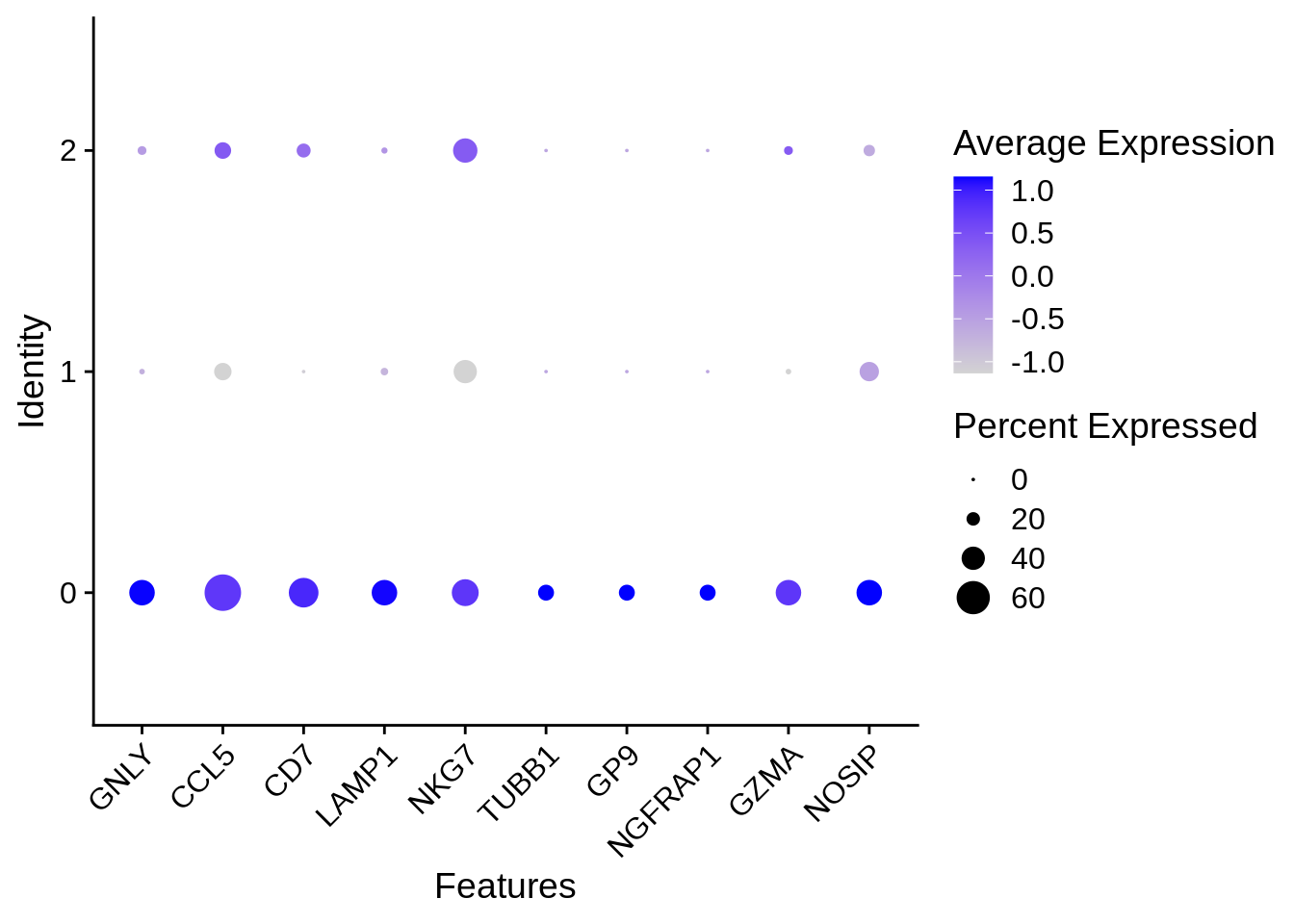
## SP100 9.699402e-03 2.3096455 0.526 0.164 1.000000e+00 2 SP100DotPlot
There is another common visualization technique that involves mapping the percent of cells that express a certain gene to the size of a dot, and color it according to the average expression value. Here’s an example:
🧭✨ Polls: How would you extract the ‘gene programme’ of a given cluster? A ‘gene programme’ would be the group of genes that are characteristic and could serve the purpose of defining such a cluster as a given celltype.
⌨🔥 Exercise: We’ll distribute the room in groups again (N<=9), and assign a cluster to each. Get the “gene signature” of your assigned cluster, see if you can assign the correct celltypes by using the following list of gene markers.
list(
  `Naive CD4+ T` = c("IL7R", "CCR7"),
  `CD14+ Mono` = c("CD14", "LYZ"),
  `Memory CD4+` = c("IL7R", "S100A4"),
  B = c("MS4A1"),
  `CD8+ T` = c("CD8A"),
  `FCGR3A+ Mono` = c("FCGR3A", "MS4A7"),
  NK = c("GNLY", "NKG7"),
  DC = c("FCER1A", "CST3"),
  Platelet = c("PPBP")
)
## $`Naive CD4+ T` ## [1] "IL7R" "CCR7" ## ## $`CD14+ Mono` ## [1] "CD14" "LYZ" ## ## $`Memory CD4+` ## [1] "IL7R" "S100A4" ## ## $B ## [1] "MS4A1" ## ## $`CD8+ T` ## [1] "CD8A" ## ## $`FCGR3A+ Mono` ## [1] "FCGR3A" "MS4A7" ## ## $NK ## [1] "GNLY" "NKG7" ## ## $DC ## [1] "FCER1A" "CST3" ## ## $Platelet ## [1] "PPBP"
Apart from getting and visualizing marker genes, we would ultimately want to see whether there are common functional themes in those marker lists. This will be covered in the next section.