Slides are here.

Setup

library(Seurat)
options(Seurat.object.assay.version = "v5")
packageVersion("Seurat")

## [1] '5.1.0'

What does the data look like out of the box?

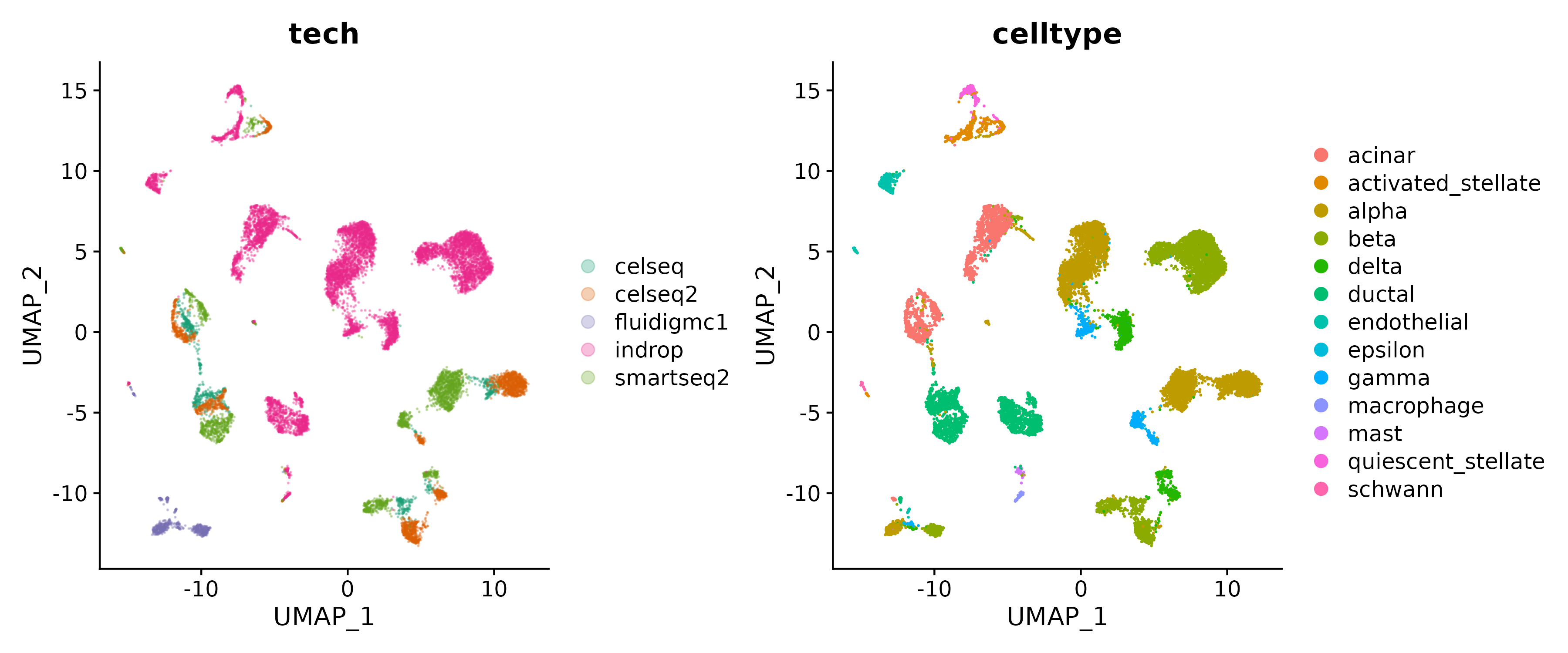
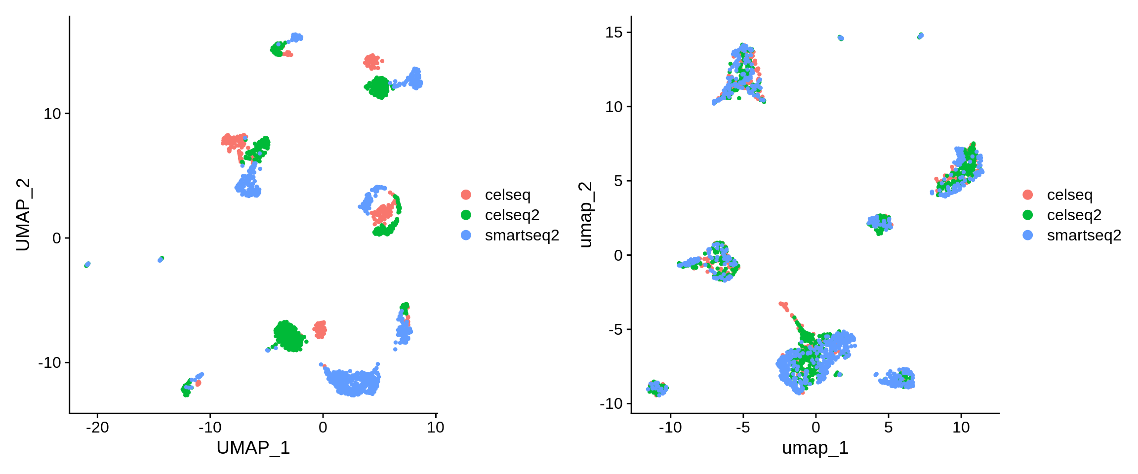
Lets have a look at the UMAP embedding of the full dataset processed in a standard way, ignoring any possible batch effects. Compare the cell separation by sequencing technology and by cell type.

Full dataset on umap

Load the preprocessed subset dataset

We have subset and pre-processed the full dataset for you. You can download it from zenodo.

fdest <- "datasets/preprocessed_rds/panc_sub_processed.RDS"

if (!file.exists(fdest)) {
    # utils::download.file('https://zenodo.org/record/7891484/files/panc_sub_processed.RDS?download=1',
    # destfile = fdest, method = 'curl')
    file.copy("/scratch/local/rseurat/datasets/preprocessed_rds/panc_sub_processed.RDS",
        fdest, overwrite = FALSE)
}
panc_sub <- UpdateSeuratObject(readRDS(fdest))  ## Seurat v5 would require this

🧭✨ Poll:

Which sequencing technologies are retained in the subset dataset?

How many cells were sequenced with smartseq2?

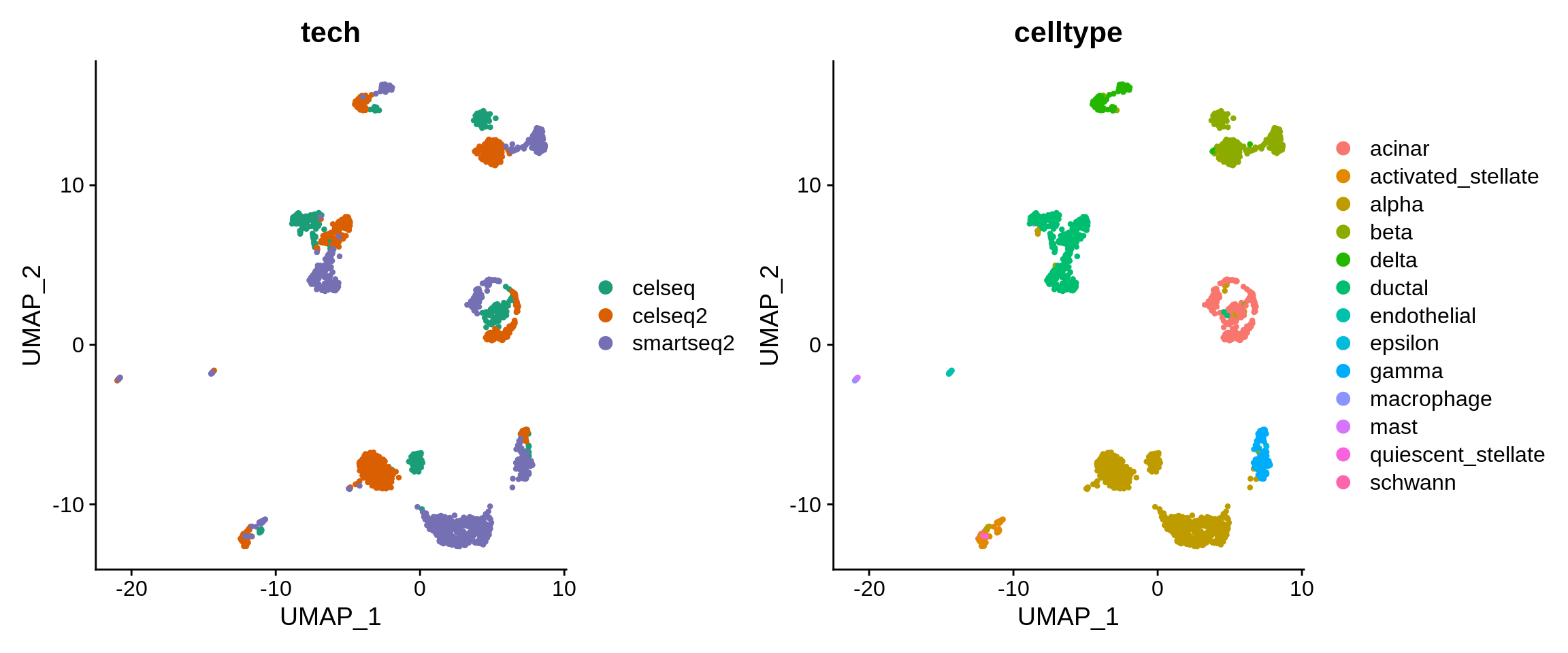
Revisit UMAP

Plot UMAP embedding for the subset dataset. Inspect the cell separation by cell type and by sequencing technology.

⌨🔥 Exercise: plot gene expression

In the previous course units, you have learned to call differentially expressed genes with Seurat. In this task, we ask you to: - call genes differentially expressed between cells sequenced with the smartseq2 technology and those with the celseq technology - plot a violin plot for the top gene - plot a feature plot for the top gene

🧭✨ Poll: What is the name of the top DE gene ?

Here’s our proposed solution:

smartseq2.markers <- FindMarkers(panc_sub, ident.1 = "smartseq2", ident.2 = "celseq",
    only.pos = TRUE)
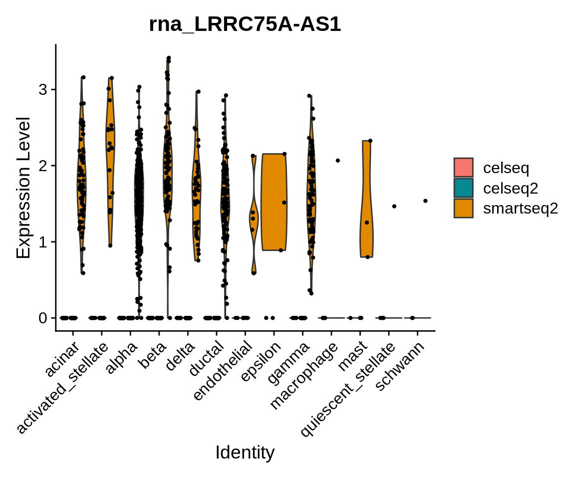
VlnPlot(panc_sub, features = "LRRC75A-AS1", group.by = "celltype", split.by = "tech",
    split.plot = TRUE)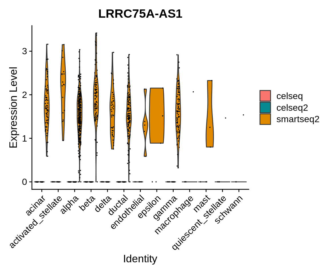

This gene appears to be mostly expressed in cells sequenced with the smartseq2 technology in multiple cell populations.

Let’s plot it’s expression on the lowD embedding:

p1 <- FeaturePlot(panc_sub, features = "LRRC75A-AS1")
p2 <- DimPlot(panc_sub, reduction = "umap", group.by = "tech", cols = scales::alpha(my_cols,
    0.3))
p1 + p2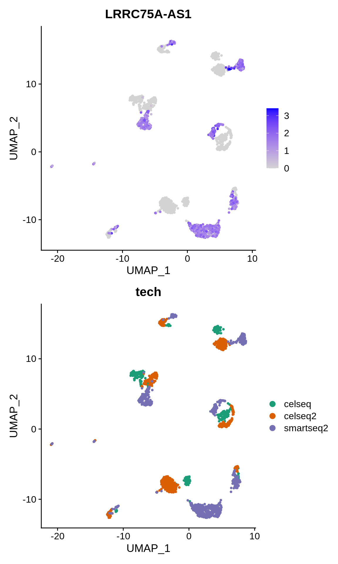

On the other hand, what does the expression of known celltype markers look like ? Let’s plot the expression of the alpha cell marker gen “GCG”.

p1 <- FeaturePlot(panc_sub, features = "GCG")
p2 <- DimPlot(panc_sub, reduction = "umap", group.by = "celltype")
p1 + p2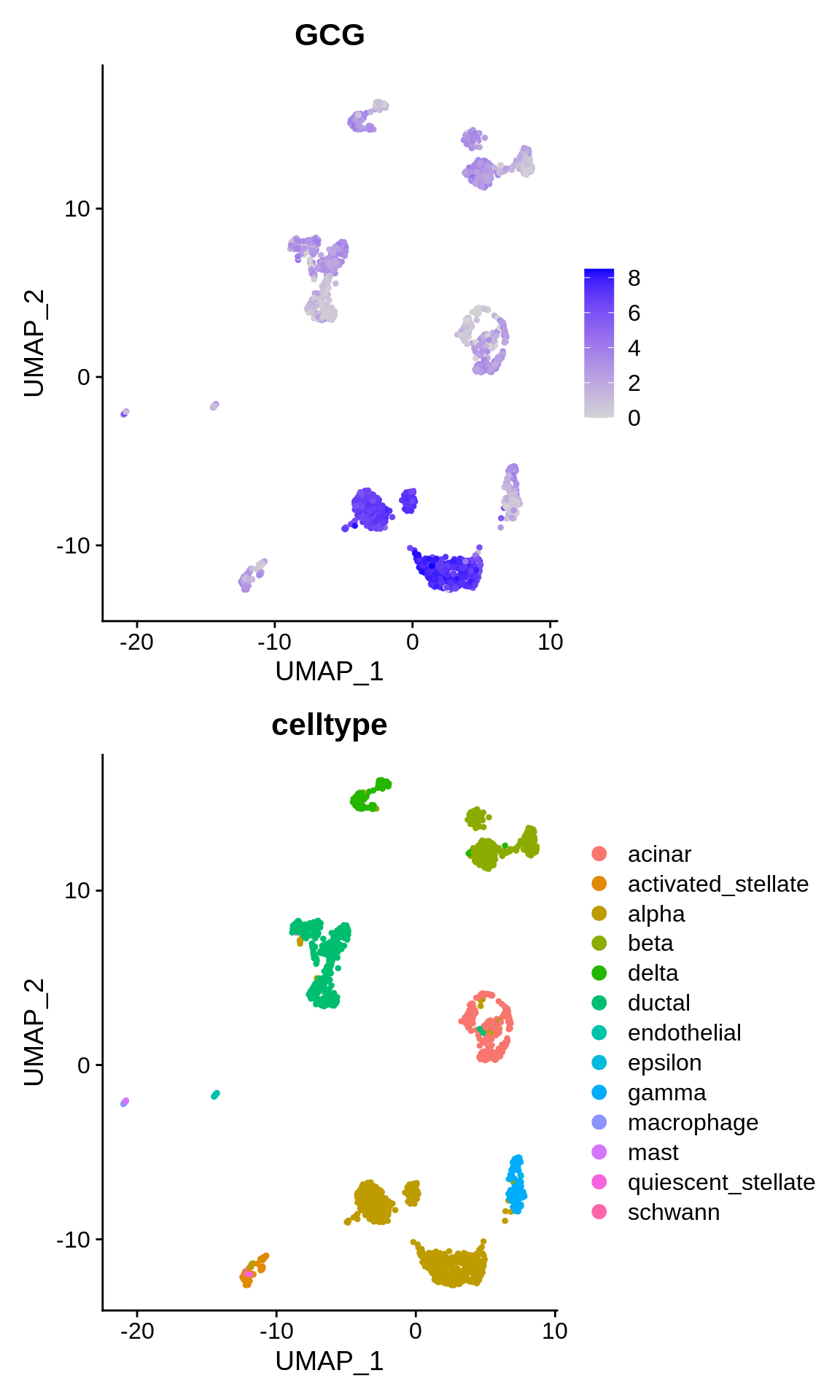

What options are there to mitigate batch effects ?

Let’s now explore some options of mitigating batch effects:

Harmony (briefly shown here)
Seurat Integration (we’ll do this next)
SCTransform (we’ll see tomorrow)
kBET
Conos
ComBat/SVA
…

Harmony

This method is quite straightforward. It will account for batch effects by correcting our principal components, its functionality is conveniently wrapped under function RunHarmony. Just keep in mind that it will create a new ‘harmony’ reduction that’s the one you want to use downstream…

The next code block illustrates the process. Unfortunately, we won’t apply this methodology here. But it should be straightforward for you to use it when/ if the need arises. For further details, check the package vignette (tutorial).

# Load DATA
obj.Name1 <- CreateSeuratObject(counts = counts.Name1, project = "Name1")
obj.Name2 <- CreateSeuratObject(counts = counts.Name2, project = "Name2")

# Merge DATA
object <- merge(x = obj.Name1, y = obj.Name2, add.cell.ids = c("Name1",
    "Name2"), merge.data = F)

## This will give you a 'orig.ident' meta-data column with 'Name1' or
## 'Name2', allowing you to know from which experiment came each
## cell.

# ... QC, etc.
harmony::RunHarmony(object, h.group.by.vars = "orig.ident")
FindNeighbors(object, reduction = "harmony")
FindClusters(object)
RunUMAP(object, reduction = "harmony")
# ... DE, etc.

Seurat Integration

There’s a few more slides, here. For further details, check the original article.

Seurat Integration: prep datasets

Prior to the integration, we want to normalize each dataset separately to be integrated.

# split the dataset into a list of seurat objects
panc.list <- SplitObject(panc_sub)

# normalize and identify variable features for each dataset
# independently
panc.list <- lapply(X = panc.list, FUN = function(x) {
    x <- NormalizeData(x)
    x <- FindVariableFeatures(x, selection.method = "vst", nfeatures = 2000)
})

Seurat Integration

# select features that are repeatedly variable across datasets for
# integration
features <- SelectIntegrationFeatures(object.list = panc.list)

anchors <- FindIntegrationAnchors(object.list = panc.list, anchor.features = features,
    normalization.method = "LogNormalize")

# this command creates an 'integrated' data assay
panc.combined <- IntegrateData(anchorset = anchors, normalization.method = "LogNormalize")

Let’s clean up some redundant objects from memory.

rm(list = c("panc.list", "features", "anchors"))
gc()

##             used   (Mb) gc trigger   (Mb)  max used   (Mb)
## Ncells   8549044  456.6   17055038  910.9  17055038  910.9
## Vcells 193155952 1473.7  502811043 3836.2 501544092 3826.5

Let’s have a brief look at the panc.combined dataset - a new Assay has been created by the integration procedure.

🧭✨ Poll: What is the new assay called? Hint: you can access assays of a Seurat object with Assays().

Process the newly integrated dataset

After the integration, data scaling on the new assay is necessary, as well as calculation of PCA and UMAP embeddings.

stopifnot(DefaultAssay(panc.combined) == "integrated")

# Run the standard workflow for visualization and clustering
panc.combined <- ScaleData(panc.combined, verbose = FALSE)
panc.combined <- RunPCA(panc.combined, verbose = FALSE)
panc.combined <- RunUMAP(panc.combined, reduction = "pca", dims = 1:30)

What does the data look like after the integration?

Let’s have a look at the distribution of technology, and celltype, labels in lowD after integration.

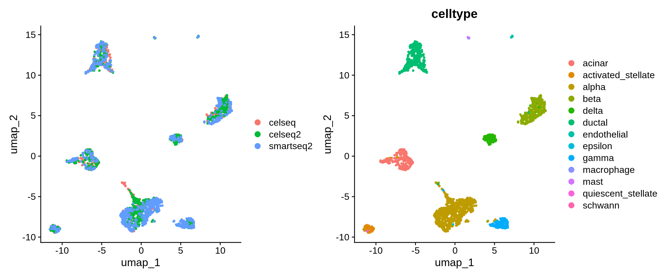
We can also compare the distribution of cell tech labels before and after integration.

⌨🔥 Exercise: plot gene expression after integration

You have previously plotted the expression of a DE gene between the sequencing technologies on the dataset before integration. Repeat the violin and the feature plot for the dataset after integration. What has changed, what hasn’t, and why?

Here’s our proposed solution:

VlnPlot(panc.combined, features = "LRRC75A-AS1", group.by = "celltype",
    split.by = "tech")

The expression of this gene hasn’t changed - as it is not present in the “integrated” assay, the VlnPlot function has fetched it’s expression value from the RNA assay, which is not modified by the integration.

Let’s plot it’s expression on the lowD embedding:

p1 <- FeaturePlot(panc.combined, features = "LRRC75A-AS1")
p2 <- DimPlot(panc.combined, reduction = "umap", group.by = "tech", cols = scales::alpha(my_cols,
    0.3))
p1 + p2

We can now appreciate that cells highly expressing this gene are distributed over all clusters. Note that the mixing with the cells negative for this marker is imperfect, but such is the result of the integration for this dataset.

Let’s ascertain ourselves that the expression of the celltype markers is behaving as expected after integration. For this purpose, let’s plot the expression of the alpha cell marker gen “GCG”.

p1 <- FeaturePlot(panc.combined, features = "GCG")
p2 <- DimPlot(panc.combined, reduction = "umap", group.by = "celltype")
p1 + p2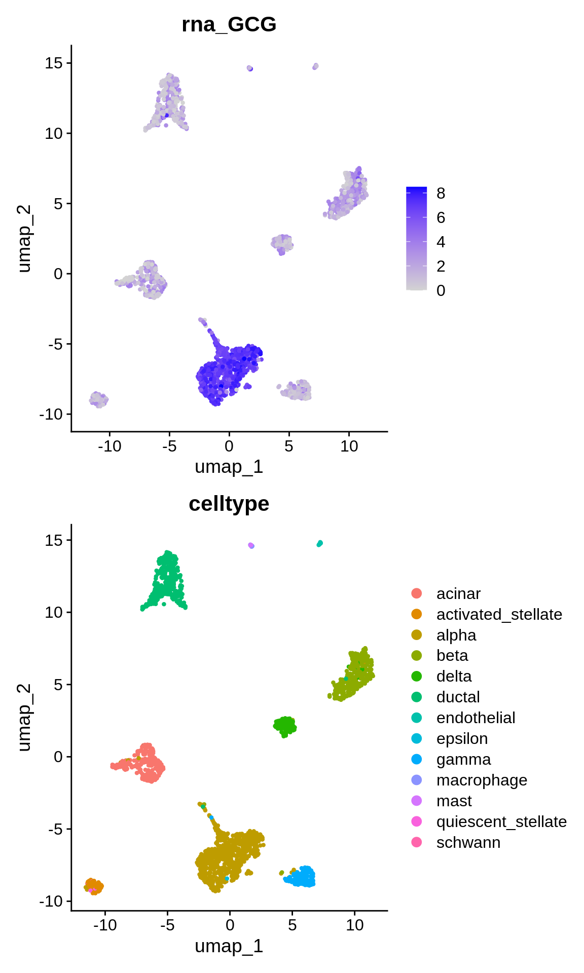

End

Citations

Büttner, M., Miao, Z., Wolf, F.A. et al. A test metric for assessing single-cell RNA-seq batch correction. Nat Methods 16, 43–49 (2019). https://doi.org/10.1038/s41592-018-0254-1

Stuart T, Butler A, Hoffman P, Hafemeister C, Papalexi E, Mauck WM 3rd, Hao Y, Stoeckius M, Smibert P, Satija R. Comprehensive Integration of Single-Cell Data. Cell. 2019 Jun 13;177(7):1888-1902.e21. doi: 10.1016/j.cell.2019.05.031. Epub 2019 Jun 6. PMID: 31178118; PMCID: PMC6687398

Appendix

This is how to reproduce generation of the UMAP embedding for the full dataset and further the generation of the subset dataset used in this course unit:


library(SeuratData)
panc <- LoadData("panc8", type = "default")
table(panc$dataset)
panc <- NormalizeData(panc)
panc <- FindVariableFeatures(panc, selection.method = "vst", nfeatures = 2000)
all.genes <- rownames(panc)
panc <- ScaleData(panc, features = all.genes)
panc <- RunPCA(panc, features = VariableFeatures(object = panc))
panc <- RunUMAP(panc, dims = 1:15)
p1<-DimPlot(panc, reduction = "umap",label=TRUE)
p2<-DimPlot(panc, reduction = "umap",group.by="celltype")
p1+p2

panc_sub <- subset(x=panc,subset = dataset == c("celseq","celseq2","smartseq2"))
panc_sub <- NormalizeData(panc_sub)
panc_sub <- FindVariableFeatures(panc_sub, selection.method = "vst", nfeatures = 2000)
all.genes <- rownames(panc_sub)
panc_sub <- ScaleData(panc_sub, features = all.genes)
panc_sub <- RunPCA(panc_sub, features = VariableFeatures(object = panc_sub))
panc_sub <- RunUMAP(panc_sub, dims = 1:15)
saveRDS(panc_sub,"panc_sub_processed.RDS")

Batch Effects

Setup

What does the data look like out of the box?

Load the preprocessed subset dataset

Revisit UMAP

What options are there to mitigate batch effects ?

Harmony

Seurat Integration

Seurat Integration: prep datasets

Seurat Integration

Process the newly integrated dataset

What does the data look like after the integration?

End

Citations

Appendix