SCTransform
Slides are here.
SeuratData
We’re going to work with IFNB-Stimulated and Control human PBMCs and downsample the datasets for the purpose of the exercise.
data(list = "ifnb", package = "ifnb.SeuratData")
ifnb <- UpdateSeuratObject(ifnb)
ifnb_sub <- subset(x = ifnb, downsample = 1000)
table(ifnb_sub$stim)
##
## CTRL STIM
## 1000 1000ifnb.list <- SplitObject(ifnb_sub, split.by = "stim")
ctrl <- ifnb.list[["CTRL"]]
stim <- ifnb.list[["STIM"]]Let’s remove some redundant objects from memory:
Standard normalization?
Lets process the control dataset in a standard way. We’re going to save the elbow plot and compare it with the one obtained on sc-trasnformed data later on.
ctrl <- NormalizeData(ctrl)
ctrl <- FindVariableFeatures(ctrl, selection.method = "vst", nfeatures = 2000)
all.genes <- rownames(ctrl)
ctrl <- ScaleData(ctrl, features = all.genes)
ctrl <- RunPCA(ctrl, features = VariableFeatures(object = ctrl))
ctrl_ln <- ElbowPlot(ctrl, ndims = "30")
ctrl <- RunUMAP(ctrl, dims = 1:15)
What does the data look like out of the box?
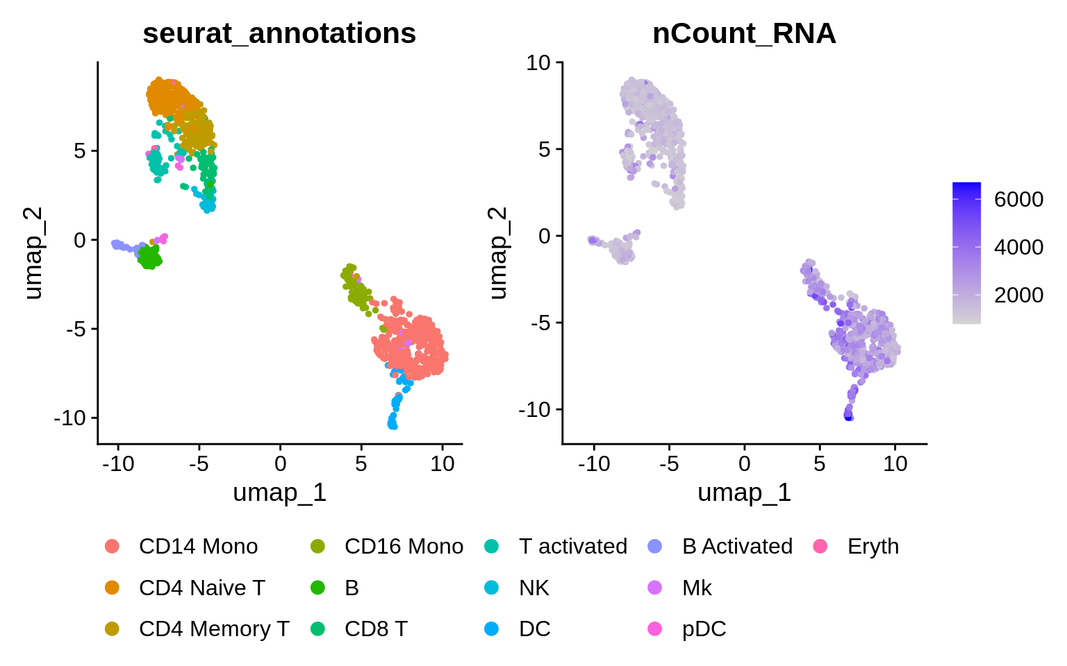
🧭✨ Poll: Which cell population has the highest total counts? Hint: use the
FetchDatato retrieve variablesnCountsandseurat_annotationsto a data frame. Process it further with Dplyr functions:group_by,summarize(total_counts = sum(nCount_RNA)), andarrange.
Seurat SCTransform
The SCTransform function performs normalization,
regressing out of nuissance variables and identification of variable
features. By default, total UMI count per cell are regressed out, but
it’s possible to add other variables to the model, e.g. mitochondrial
gene content.
We’re going to use the SCTransform function with some more recent implementations of NB modelling and variance stabilizing transformation.
# This is only needed for those students that run the installation
# script as it was sent out by email. Pick ONLY one solution, the
# second could be better.

# remotes::install_version('matrixStats', version='1.1.0')
# remotes::install_github('Bioconductor/MatrixGenerics@RELEASE_3_18')We could’ve also regressed out covariates during this process.
Recalculate Dimensional Reductions
We have now gotten a new Assay added to the Seurat object. All we need to do now is to run PCA and UMAP for visualization in lowD. We’re also going to save the elbow plot for comparison with the log-normed dataset.
stopifnot(DefaultAssay(ctrl) == "SCT")
ctrl <- RunPCA(ctrl, verbose = FALSE)
ctrl_sct <- ElbowPlot(ctrl, ndims = "30")
Let’s compare the elbow plots for the dataset normalzed with either of the two methods:
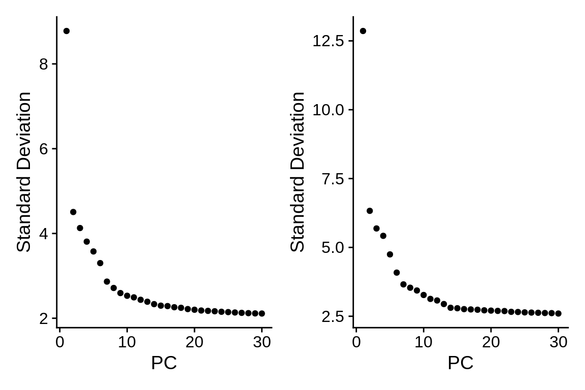
What has changed and what hasn’t?
🧭✨ Poll: What amount of standard deviation does PC1 explain after sc-transform? Hint: Function
Stdev(object)returns the absolute values of standard deviations for principal components. It’s the analogous toobject@reductions$pca@stdev.
Revisit UMAP
We can choose more PCs when using sctransform to calculate the lowD embedding. The authors believe this is because the sctransform workflow performs more effective normalization, strongly removing technical effects from the data. Higher PCs are more likely to represent subtle, but biologically relevant, sources of heterogeneity – so including them may improve downstream analysis. We’re going to use 30 top PCs to calculate the UMAP embedding in the SCT assay.
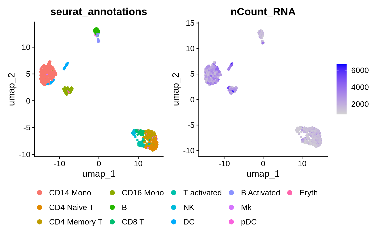
What has changed and what hasn’t ?
⌨🔥 Exercise: Apply SCTransform to the IfnB-stimulated dataset as well.
🧭✨ Poll: What amount of standard deviation does the first PC explain after applying sc-transform to the stimulated dataset?
Prepare both datasets for integration
We’re now going to revisit dataset integration after sc-transform. We can now select 3000 features for integration, instead of the default 2000 in case of log-normalized data. SC-transformed data requires an additional preparation step prior to integration. This performs sanity checks i.e. that sctransform residuals specified in to anchor.features are present in each object of the list; subsets the scale.data slot to only contain the residuals for anchor.features.
stim <- SCTransform(stim, method = "glmGamPoi", vst.flavor = "v2", verbose = FALSE) %>%
    RunPCA(npcs = 30, verbose = FALSE)
ifnb.list <- list(ctrl = ctrl, stim = stim)
features <- SelectIntegrationFeatures(object.list = ifnb.list, nfeatures = 3000)
ifnb.list <- PrepSCTIntegration(object.list = ifnb.list, anchor.features = features)
Seurat Integrate
The datasets are now ready for integration. The same two steps are used as for a log-transformed dataset. There is a slight difference of what the function returns, though. If normalization.method = “LogNormalize”, the integrated data is returned to the data slot and can be treated as log-normalized, corrected data. If normalization.method = “SCT”, the integrated data is returned to the scale.data slot and can be treated as centered, corrected Pearson residuals.
immune.anchors <- FindIntegrationAnchors(object.list = ifnb.list, normalization.method = "SCT",
    anchor.features = features)
immune.combined.sct <- IntegrateData(anchorset = immune.anchors, normalization.method = "SCT")
## [1] 1
## [1] 2Let’s cleanup again:
Process the newly integrated dataset
All we need to do now is to run PCA and UMAP on the integrated assay.
What does the data look like after the integration?
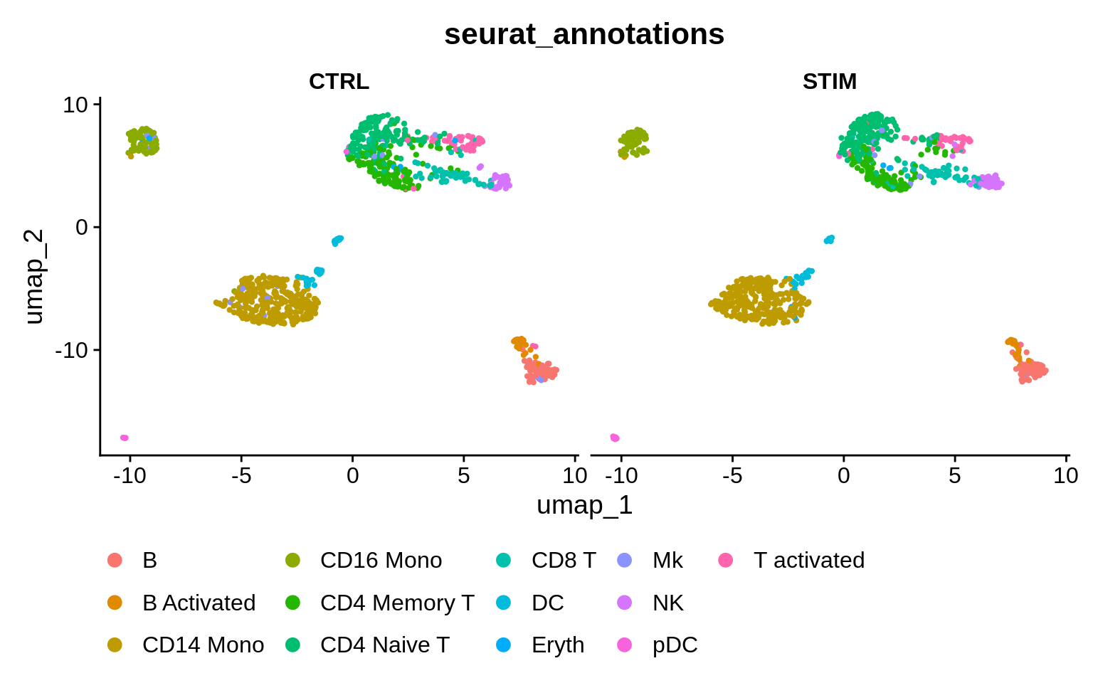
It appears that both conditions are contributing to all clusters, as no condition-specific clusters are apparent. How would you go about checking the percentages of cells from each condition in each cluster?
DE genes
We’re now going to run DGE analysis on the SCT assay, with the goal of getting a list of top 10 DE genes between stimulated and unstimulated B cells. First, we’re going to rename cell identities to a concatenation of celltype and condition.
As we’re going to test across conditions, the datasets for which have
been sc-transformed separately (multiple SCT models), we’ll have to
invoke PrepSCTFindMarkers before we can run the
FindMarkers function. This is going to recorrect the counts
in the count slots using minimum of the median UMI of
individual objects to reverse the individual SCT regression models.
FindMarkers is going to use the recorrected
count slots.
immune.combined.sct$celltype.stim <- paste(immune.combined.sct$seurat_annotations,
    immune.combined.sct$stim, sep = "_")
Idents(immune.combined.sct) <- "celltype.stim"
immune.combined.sct <- PrepSCTFindMarkers(immune.combined.sct)

b.interferon.response <- FindMarkers(immune.combined.sct, assay = "SCT",
    ident.1 = "B_STIM", ident.2 = "B_CTRL", verbose = FALSE)
head(b.interferon.response, n = 10)
⌨🔥 Exercise: Plot SCT “corrected counts” for one of the DE genes on a lowD representation, splitting by the stimulation status.
Proposed solution
Idents(immune.combined.sct) <- "seurat_annotations"
inf_genes <- rownames(b.interferon.response)
DefaultAssay(immune.combined.sct) == "SCT"  # integrated
## [1] FALSEFeaturePlot(immune.combined.sct, features = inf_genes[1], split.by = "stim",
cols = c("grey", "red")) + theme(legend.position = "right")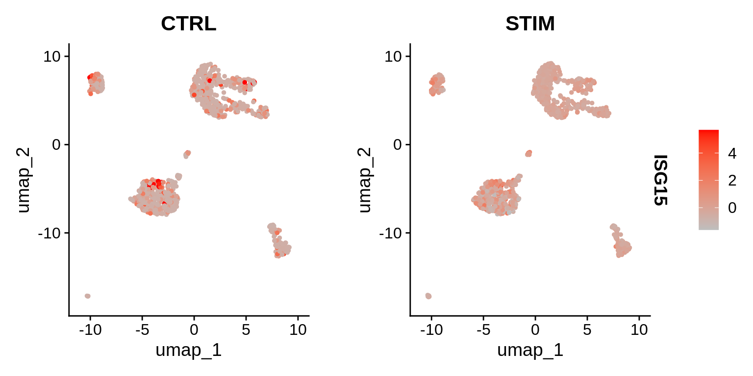
FindConservedMarkers
You may also want to identify markers that are DE between identities
independent of the conditions. For that purpose, you can make
use of the FindConservedMarkers function. The
PrepSCTFindMarkers command does not to be rerun here.
End
Citations
Hafemeister, C., Satija, R. Normalization and variance stabilization of single-cell RNA-seq data using regularized negative binomial regression. Genome Biol 20, 296 (2019). https://doi.org/10.1186/s13059-019-1874-1
Choudhary, S., Satija, R. Comparison and evaluation of statistical error models for scRNA-seq. Genome Biol 23, 27 (2022). https://doi.org/10.1186/s13059-021-02584-9
Ahlmann-Eltze C, Huber W (2020). “glmGamPoi: Fitting Gamma-Poisson Generalized Linear Models on Single Cell Count Data.” Bioinformatics. doi: 10.1093/bioinformatics/btaa1009, https://doi.org/10.1093/bioinformatics/btaa1009.