Functional Analyses
Setup
# .libPaths(new = "/scratch/local/rseurat/pkg-lib-4.2.3")

suppressMessages({
  library(enrichR)
  library(tidyverse)
  library(Seurat)
})


set.seed(8211673)

knitr::opts_chunk$set(echo = TRUE, format = TRUE, out.width = "100%")


options(
  parallelly.fork.enable = FALSE,
  future.globals.maxSize = 8 * 1024^2 * 1000
)

plan("multicore", workers = 8)
## work directory: /home/runner/work/Rseurat/Rseurat/rmd## library path(s): /home/runner/micromamba/envs/Rseurat/lib/R/libraryLoad Data
We’ll be working with the data from our past notebook (“First steps”), let’s quickly re-load and re-process again:
pbmc <- Read10X(data.dir = "./datasets/filtered_gene_bc_matrices/hg19/") %>%
  CreateSeuratObject(counts = ., project = "pbmc3k", min.cells = 3, min.features = 200)

pbmc[["percent.mt"]] <- PercentageFeatureSet(pbmc, pattern = "^MT-")

pbmc <- subset(pbmc, subset = nFeature_RNA > 200 & nFeature_RNA < 2500 & percent.mt < 5)

pbmc <- NormalizeData(pbmc, verbose = FALSE)

pbmc <- FindVariableFeatures(pbmc, verbose = FALSE)

pbmc <- ScaleData(pbmc, features = rownames(pbmc), verbose = FALSE)

pbmc <- RunPCA(pbmc, features = VariableFeatures(pbmc), verbose = FALSE)

pbmc <- FindNeighbors(pbmc, dims = seq_len(10), verbose = FALSE)

pbmc <- FindClusters(pbmc, resolution = 0.5, verbose = FALSE)

pbmc <- RunUMAP(pbmc, dims = seq_len(10), verbose = FALSE)
## Found more than one class "dist" in cache; using the first, from namespace 'spam'## Also defined by 'BiocGenerics'## Found more than one class "dist" in cache; using the first, from namespace 'spam'## Also defined by 'BiocGenerics'Next, we do our between-clusters DE analysis:
markers.between.clusters <- FindAllMarkers(
  pbmc_small,
  test.use = "MAST",
  logfc.threshold = 0.125,
  min.pct = 0.05,
  only.pos = TRUE,
  densify = TRUE
)
## Calculating cluster 0##
## Done!## Combining coefficients and standard errors## Calculating log-fold changes## Calculating likelihood ratio tests## Refitting on reduced model...##
## Done!## Calculating cluster 1##
## Done!## Combining coefficients and standard errors## Calculating log-fold changes## Calculating likelihood ratio tests## Refitting on reduced model...##
## Done!## Calculating cluster 2##
## Done!## Combining coefficients and standard errors## Calculating log-fold changes## Calculating likelihood ratio tests## Refitting on reduced model...##
## Done!Functional Enrichment Analysis
These methods have first been used for microarrays, and aim to draw conclusions ranked gene list from RNAseq experiments, scRNA, or any other OMICS screen. There are a number of tools and approaches - here we will focus only one common and practical approach.
For more information, see: clusterProfiler.
The aim is to draw conclusions as to what’s the functional implications that we may be able to derive given a list of genes. To this end, we’d start with such list and then consult databases for the annotations. With this data, we can come up with scores to measure level of association. A gene set is an unordered collection of genes that are functionally related.
Gene Ontology
GO Terms are semantic representations in a curated database that defines concepts/classes used to describe gene function, and relationships between these concepts. GO terms are organized in a directed acyclic graph, where edges between terms represent parent-child relationship. It classifies functions along three aspects:
- MF: Molecular Function, molecular activities of gene products
- CC: Cellular Compartment, where gene products are active
- BP: Biological Processes, pathways and larger processes made up of the activities of multiple gene products
enrichR
The package is already loaded. But we need to select which databases
to connect. There are more than 200 databases available, you can get a
data frame with details of these using listEnrichrDbs().
For this and the following to work you need a working internet
connection.
dbs <- c(
  "GO_Biological_Process_2023",
  "GO_Cellular_Component_2023",
  "GO_Molecular_Function_2023"
)## Uploading data to Enrichr... Done.
## Querying GO_Biological_Process_2023... Done.
## Querying GO_Cellular_Component_2023... Done.
## Querying GO_Molecular_Function_2023... Done.
## Parsing results... Done.⌨🔥 Exercise(s):
- Understand the format and interpret the output
result.1.- What is the most significantly enriched molecular function? which genes are the base for it?
- Would you get the same result if you changed the number of marker genes in the input? Try it out.
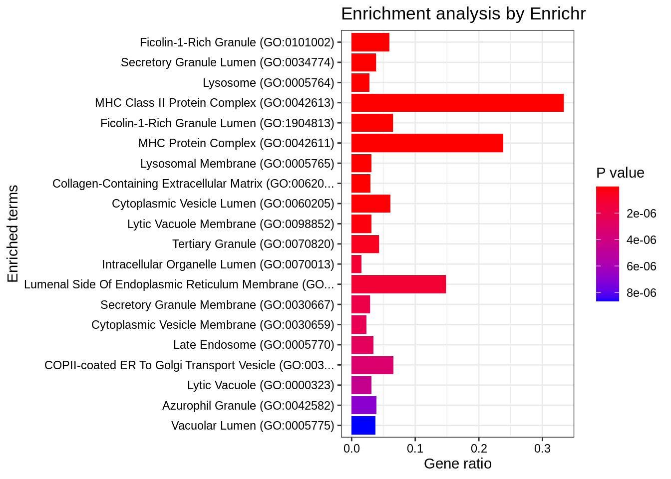
We can also produce nice graphical summaries:
Also, we may customize the selection and subsetting of top ranking categories that are visualized:
result.1$GO_Cellular_Component_2023 %>%
  filter(
    Adjusted.P.value < 5e-2,
    Odds.Ratio != 1
  ) %>%
  arrange(-Combined.Score) %>%
  # Combined.Score = ln(p)*z
  plotEnrich(showTerms = 20, numChar = 50, y = "Ratio")